from JBAA 110, 3, 2000 June
R Aquilae is well known as a Mira variable of ever decreasing period. Statistical tests upon, and descriptive analyses of, this star are conducted. Conclusions are drawn regarding the significance of R Aquilae's variation in period. Since this star's change in period is so conspicuous, it serves as a baseline against which the results for other Miras can be compared.
R Aquilae = HR 7243 = HD 177940 = SAO 124266 = HIP 93820 = TYC/GSC 1040 0241 1 is a Mira type variable listed3 as ranging from mv 5.5 to 12.2 and M5e - M9e III in spectral type. It has a mean B-V index of +1.144 and a trigonometric parallax of ~ 0.005" Although listed as the multiple star Ball 365 with mv 11.1 and 10.5 comites lying at 76.6" and 180.7" in position angles of 297° and 259° respectively, the two companion stars have quite dissimilar proper motions to R Aquilae and are probably only optical comites.
Several methods have been suggested in the past to test trends in Mira variable periodicity for any statistical significance. At the outset it should be noted that statistical tests are usually those of the null hypothesis, which in the following case is the hypothesis that the variation in periodicity under examination is purely random. If the tabulated value for the (say) 0.05 probability for the null hypothesis is exceeded, then it can be inferred that the data is representative of a genuine trend.
In other words, the probability of such a value arising for the test statistic by pure chance under the null hypothesis would be less than 0.05 (5% if preferred), giving strong evidence for a genuine nonrandom effect. Such a result is referred to as being significant to better than the 0.05 level. Tables normally give the significance threshold values for the 0.05, 0.02, 0.01 and 0.001 null hypothesis probabilities, though other threshold values can sometimes be given. It should always be remembered, however, that these are tests upon the data, and although their results are highly suggestive, they do not say anything with regards to the physical system(s) under investigation. Statistics are also highly dependent on the questions being asked, and should never be quoted out of context.
The earliest statistical test involved the derivation of periods between known times of maxima or minima and their binning into groups of ten or more cycles. These are then tested to see which bins, if any, have an excess of periods above or below the mean. This is Sterne's c2 test.6
The span length test7 was introduced in a series of papers by Isles and Saw who were investigating a number of Mira variables that had data in the BAAVSS archive. The method uses the output from an O-C (Observed minus Calculated) examination of the observations for a star, which involves the derivation of maxima from a light curve, and the calculation of the residuals between these observed maxima and those calculated from a base epoch and test period. In Isles' and Saw's formulation7 of the O-C the test period was defined as the mean interval between first and last epoch divided by the number of cycles [i.e. (tn-t0)/n]. The maximal deviation in O-C residual (whether positive or negative) is then taken, and its absolute value divided by the sample standard deviation (s) of the periods (i.e. intermaxima intervals). The resultant test statistic is then checked against tables.8 This method owes an allegiance to cumulative sum procedures, or CUSUMs.
Isles & Saw went on to investigate stars using the correlation coefficient between successive periods.9 Here the correlation between a list of periods is checked against the same list offset by a certain number of positions along the list; this offset is the lag. As Isles & Saw point out, the time of maximum marking the end of one period is the same as the one marking the beginning of the next, thus consecutive periods are not truly independent, which leads to an inherent negative correlation between consecutive periods. They therefore used a lag of 2: i.e. each period from the list was tested for correlation against the next but one period in the same list. The resultant value can be checked against tables of Pearson's sample correlation coefficient (r) for its significance, the degree of freedom being defined as the number of pairs compared minus 2, a two-tailed normal distribution being assumed here.
Lloyd10 gives a general overview of these methods, with further references, whilst extending the way they can be used. Firstly he suggests that the methods in question should be followed in an 'evolutionary' or 'historical' manner. Consequently, the above statistics are taken for subsets of the complete data starting at the 20th cycle, by which time the behaviour of the star's data should be fairly well established. The statistical significance is then taken for cycles 20, 21, 22, ..., n (where n is the number of the last cycle) and plotted against the appropriate cycle number. It is also informative to include lines of constant significance upon the plot. Although statistical in nature, these plots are also quite useful descriptively, and could equally as well have been mentioned in the next subsection.
Secondly, he suggests extending the lag 2 correlation methodology to ever increasing lags, that is calculating the autocorrelation function of the periods, and plotting the results on a correlogram. Again, this is just as much a descriptive as a statistical procedure, as the correlogram can contain a great deal of information.
All the above methods have one fairly important limitation: they are only really most productive when detecting monotonic trends in variation. If a run of data should consist of cyclical variations such that said cycles occur twice or more within the run, then these variations are liable to be unseen by the above tests, or at least not shown in a clear cut way.
Finally, Koen and Lombard (KL) in a series of papers11,12,13 suggest new methods of testing for real variation in periodicity, pointing out the failure of most traditional methods due to their incorrect handling of (or even complete ignoring of) the trend in the errors. As the periods are random the O-C residuals suffer random walks and although obviously random in nature the effect of these latter are cumulative. Any early trend in variation can persist later into the investigation, and not necessarily be 'washed out' in the relatively short term.
One simple aspect of KL's work is somewhat analogous to an above mentioned technique. This is the so called 'portmanteau' statistic Q,11 defined as:
Q = N S rk2
where N is the number of observations, k the lag, and r Pearson's sample correlation coefficient. In essence rk is generated during construction of the correlogram (above). The difference here is that Q is stated as being distributed approximately as c2 with j degrees of freedom. KL state that taking Q for j (effectively the value of the maximal lag used) of around 10 or 15 is a fairly reasonable test of significance.
The self-evident and persistent decline in period exhibited by R Aquilae is useful for the evaluation of some of these statistical tests, in that should any of them fail to show evidence for any such behaviour, their efficacy is placed in question. Further, the test values derived will enable the values found for other stars to be placed in context. It will be seen that although many tests indicate very high significance for change in the period of R Aquilae, the test statistics derived are still quite modest in size, reflecting the asymptotic nature of the statistical distributions.
Descriptive
The basic descriptive tool is the simple light curve. Many Mira stars, though of high regularity, have unrepeating light curves, with variation in amplitude, period, and phenomena such as humps moving up and down the rising branch, often being much in evidence. Indeed, it is the fact that Mira stars are not regular in period, amplitude or both, which is often the main area of investigation. Many have asymmetric lightcurves, such that the rise to maximum takes less time than the decline to minimum: for others the reverse is true. The mostly random nature of this variation can be seen by the fact that the standard deviation of the periods for Mira stars is usually equivalent to 3% to 5% of the mean period. Any systematic deviation from the mean may well be less than this.
The usual first step in analysis of Mira variables is the derivation of times of maximum light. Several methods exist, including fitting polynomial curves, as with the AAVSO, or finding the point of maximum brightness from more subtle, almost hand drawn, curve fitting. When done accurately these times of maxima should be within ten days of the true date. However, as long as due care is taken in their derivation, the only thing that really matters is that the maxima are derived via a consistent procedure, so that they are readily inter-comparable.
These data can be used directly to derive periods by simply taking the interval between two consecutive maxima. A maximum to maximum interval is usually known as a cycle, and indexed in increasing numerical order from the base cycle, 0, defined here by the first derived maximum (often referred to as the Base Epoch). A simple plot of these periods against their cycle numbers can give a quick illustration of any putative trends in the data, especially if the points are joined by connecting lines and a moving average fit superposed.11
Gaps in data are a serious problem, and data suffering from too many of these is practically useless. Some mention is occasionally made of filling in gapped data via interpolation. Such averaged assumptions ignore the scatter inherent in Mira variable periods. A point to remember is the fact that many Miras show consecutive periods that are negatively correlated (i.e. longer than average periods tend to be followed by shorter than average ones and vice versa) and although this too could be taken into account, it is not a hard and fast rule. A good illustration of the potential problems would be to remove one or two periods from a data set, interpolate replacements, and then compare the results with the original true values.
The next, and usual, step is to create the O-C (Observed minus Calculated) diagram. Here a base epoch (the first derived time of maximum) is used to generate a set of observed minus calculated residuals derived by subtracting the calculated times of maxima (equal to the current cycle number multiplied by the test period, which is then added to said base epoch) from the measured (observed) times of maxima. (It can be used for minima too). The test period can be derived in several ways: either averaging over the full times of maxima and dividing by the number of cycles spanned; Discrete Fourier Transformation (DFT) of the data in a period search (see later); using catalogue values for the period (e.g. reference 3); or simply picking a suitable number out of thin air.
The O-C is primarily a linear regression technique for finding the period and base epoch. If a best fit line to the O-C residuals is horizontal then the test period is the true period; if it intersects the O-C axis at zero, then we also have the base epoch. When these two criteria are not met by any particular test period and/or base epoch, linear regression can be employed to find the appropriate corrections to these test values such that the criteria are met. In this way elements can be derived to allow for the prediction of future times of maxima [via predicted maximum's Julian date = base epoch Julian date + (test period in days x cycle number)].
Once an O-C diagram has been generated it can in principle be used to describe how the star's period has deviated from this core value over time. A decline in the value of the O-C residuals shows that the periods are shorter than the mean and maxima are occurring earlier (O is smaller than C). An increase depicts longer than average periods and later maxima (O is bigger than C). A stepwise jump along the direction of the O-C axis suggests a change in epoch.
It could be assumed, therefore, that examination of a completed O-C plot for a Mira star would result in a history of the behaviour of its period. Unfortunately, due to the aforementioned difficulties with random errors (inherent in both measurement and procedure), and the fact that the variation in the case of Miras is itself somewhat random in nature, it is often difficult to decide whether these variations are real or unreal. The O-C on its own is no proof of variation. It needs to be used in tandem with either other descriptive methods or statistical tests or, preferably, both. Even then the evidence is still only circumstantial.
Increasingly, especially with ever faster home computers, large archival data sets are being processed in toto using Discrete Fourier Analysis. Howarth gives an algorithmic procedure for this during an investigation of the periodicities of the Mira variable T Cassiopeiae.14 Such investigations are effectively a means of fitting sine waves of known period to sequentially timed data that consists of one variable quantity. Observations of a variable star, ordered by Julian date with each Julian date connected to the variant magnitude value at that date, are ideal candidates for such procedures. Problems can occur for stars that cannot be well represented by a single sinusoidal light curve, but quite a few Mira lightcurves are close enough to such a curve for this not to matter. Other problems arise with aliasing, a phenomenon where periodic gaps in the data or seasonal effects or both show signals of their own. Again, most Mira stars have a sufficiently strong main peak due to their large amplitudes, that is a sufficiently stable core periodicity, such that these other peaks usually pale into insignificance by comparison.
The converse to this is that should a well-observed Mira star with dense data and few gaps provide a cluster of closely spaced peaks instead of one peak, then there is a suggestion of period variation. If the data is good and the peak is surrounded by two fairly close lying satellite peaks, then it may well be that the period varies along a small range about a mean value. If the peaks are asymmetrical then a unidirectional trend in period variation is one possible reason. Note that these things are only suggested. The method provides no proof about the reality of these periods, or any variation therein. Indeed, it is merely pointing out signals inherent in the data, and cannot say anything about the reality of these signals with respect to actual physical processes.
The alias problem can be resolved in the case of periodic gaps and seasonal interruptions by examination of the Spectral Window Function. In this instance the time regime of the observations is examined by taking a Discrete Fourier Analysis of the data with the times unaffected but with the magnitudes set to unity, thus weighting the data set. In such situations the main period should be depicted by a strong central peak at a frequency of zero cycles per day, with any other peaks representing periodicity within the timing of the observations. It should be noted that these periods are inherent in the data and represent the relative spacing of the times of observation. For example, with a seasonally observed star the data set will contain annual gaps in the observations, which will be reflected by a peak near to or at 365.25 days.
A relatively new and considerably more in depth investigation has been devised by Howarth, known as the 'moving window' examination. 14,15 In this paper it will be referred to as the AMPSCAN procedure. The data set is first transformed into a set of n-day means to remove any artificial weighting due to over sampled regions of time. That is, each magnitude value falling within every n days is averaged and a value retained at the average date for that bin, thus each date has only one magnitude representing it, rather than a variable number as is the case with raw data. This also serves to reduce the problems caused by discrepant observations.
The data is then copied into overlapping bins which are sampled by a 'moving window' of appropriate size, such that each bin is sampled many times. A plot of phase (in degrees) against time ensues, which when inverted is directly analogous to an O-C chart (a shorter than average period causes the next cycle to be hit at a later phase, so the value in degrees increases, whereas the O-C residual decreases as the observed maximum occurs earlier compared to the calculated one).
A great advantage of this method is its high resolution. The complete light curve is being investigated, not just some arbitrarily selected representative point, which is basically all that the time of maximum is. Further, a tighter result ensues (i.e. one with less scatter), because there are no observational and/or human measurement errors involved as is the case when maxima are derived, there always being some level of subjective decision with respect to the value of maximum chosen (no matter how rigorous and honest the determination, there is still a subjective aspect involved in deciding which method to use in order to determine times of maximum/minimum). Some of this tightness, however, merely results from smoothing of the data during, and via averaging prior to, the procedure. The AMPSCAN method is somewhat reliant on a fairly complete data set, serious gaps in data giving spurious results for those times. Fortunately, the results generated at these gapped times can be filtered out, whilst the results at other times remain unaffected by this filtering.
A major bonus of this procedure is that it also shows the evolution of amplitude over time, a topic which is rarely considered in variable star analysis. There is a large emphasis on time series analysis in variable star research, for although this in itself is quite complicated most of the time, it is at least relatively easy to do and understand.
The results from such an analysis are also well illustrated by combining them into a complex phase space of two dimensions. Here the phase variation and amplitude variation are combined via x=amp X cos(phase) and y=amp X sin(phase). Radial variation within an x-y plot of this data will be representative of amplitude shift, whilst any transverse travel in the data points will be representative of phase (and consequently period) shift.
Summary
Evidently a plethora of statistical and descriptive methods can be used in the investigation of Mira star observations. None, however, has any more validity than any other in this particular context. Indeed, none even provide proof of what they reveal. Some merely test, yes or no, for a specific trend inherent in the star's visual data. Others allow the behaviour of the star's data to be followed over time, yet allow no means of separating this behaviour from purely random drift.
It is felt that as many procedures as possible should be used upon Mira star visual data, and that these procedures should be as independent as possible in their formulation. Many Mira stars show little if any sign of systematic behaviour, trends often being subtle and difficult to extract from the background random variation.16 Thus the following investigations reveal the cases for R Aquilae, a more or less self-evident instance of period and amplitude variation.
The times of maxima and the periods in days derived in reference 2 are shown in Table 1, and are the core of many of the following statistical and descriptive analyses. The base epoch (equal to cycle 0) is defined as JD 2418213.0 (or 12h UT on 1908 September 28) and maxima are derived for 104 of the 109 cycles that occurred up to 1997.
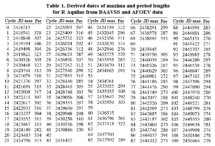
The mean of the periods is 296.3 days and the standard deviation is 17.4, that is 5.9% of the mean and therefore only slightly larger than the usual case for Miras. The median of the periods is 295.5 days, indicative of only a slight asymmetry in the distribution. The modal period of 315 days, however, reveals that there is still a strong clustering of data away from these central values. There is consequently a skew of 0.23 towards longer periods, and the negative kurtosis of -0.30 indicates that the distribution is flatter than would be the case for the normal or Gaussian distribution.
Statistics
Sterne's c2 test applied to the times of maxima in Table 1 gives a significance of 0.013 for the null hypothesis of random variation, i.e. very nearly significant at the 0.01 level. In comparison, 90+ years of BAAVSS data for c Cygni, s amounting to 85 complete cycles, reveal a significance of 0.596 for the null hypothesis, which gives no reason to suppose that the variation in the data for that period is anything but random in the case of c Cygni.
The span length test statistic is 32.8, derived from a maximal O-C residual of 576 and a sample standard deviation, s, of 17.6 for the period distribution. This maximum O-C originates from using the averaged intermaximal value of 295.9 days for the test period [(JD 2450464 - JD 2418213)/109 cycles]. For a span of 110 cycles, tables8 reveal threshold values of 13.5, 16.3 and 17.2 for the null hypothesis significances of 0.05, 0.01 and 0.005 respectively: therefore it can be safely assumed from a test value of 32.8 that the significance of random variation in the data is much better than the 0.005 level. Again for c Cygni a statistic of only 5.3 is derived, giving a 0.75 chance19 of the variation being random.
Lag 2 correlation reveals a coefficient, r, of 0.647, which amounts to a significance better than the 0.000001 level for random variation. Again, c Cygni18 gives an equivalent value of 0.037 for the null hypothesis, still significant at better than the 0.05 level, but not as dramatically so as in the case of R Aquilae.
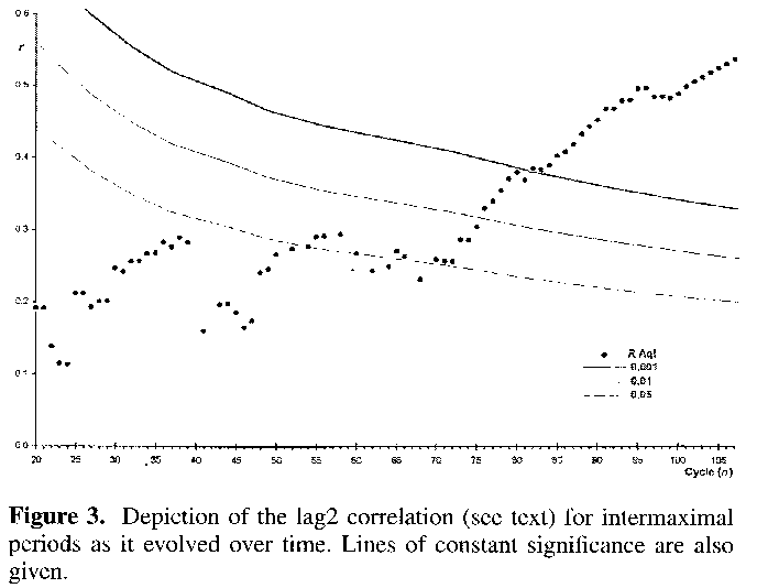
Figure 3 shows the result of extending the lag 2 correlation over time, starting at cycle twenty to give sufficient data for meaningful pair-wise comparisons. Lines of null hypothesis constant significance are shown for the 0.05, 0.01 and 0.001 levels and it can be seen that as time progresses (as cycle number and therefore number of maxima increase) the test shows ever greater significance for nonrandom variation in period. A similar plot for c Cygni rarely crosses the 0.05 line of constant significance, and never crosses the 0.01 line.
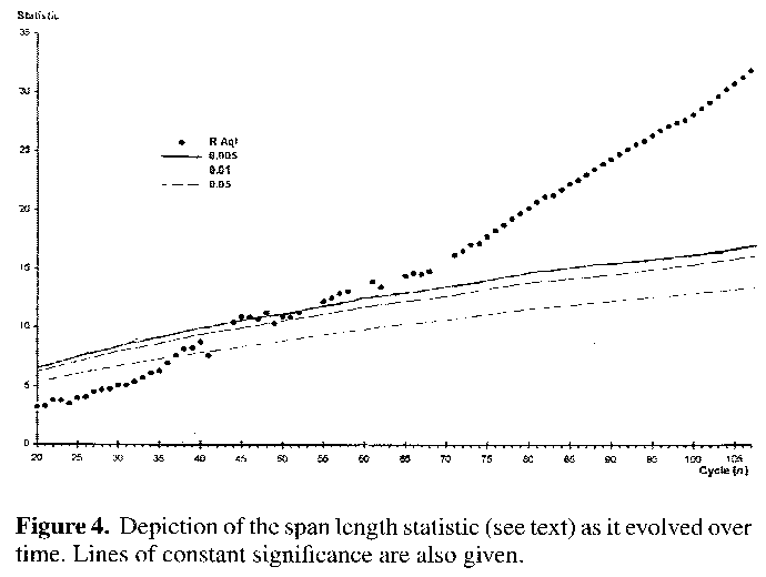
Evolving span length tests are somewhat more tedious to compile, as the average period and subsequent unique set of O-C residuals have to be derived for each progressive cycle in order to obtain the maximal residual at that point in time. Nevertheless, one such plot was generated for R Aquilae, and it can be seen from Figure 4 that the results again soon pass into areas of statistically significant nonrandom variation. A similar chart derived from 90 consecutive maxima of T Cephei16 occasionally drifts into the better than 0.05 level, actually just managing to transcend the 0.005 line at one point, but nowhere near as dramatically so as does R Aquilae. (T Cephei is believed to show some variation in period, although it is likely that this variation is somewhat cyclical, or at least bi-directional, thus lessening the utility of these statistics in its case).
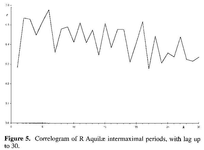
No attempt was made to create an evolving c2 plot, but the periods were used to generate a correlogram with lags up to 30, as shown in Figure 5. A high positive correlation is maintained throughout, indicative of a trend in variation: which in this case is a constant decline in period. In comparison T Cephei16 begins with strong positive correlation, only to end with strong negative correlation by lag 30 (highlighting the fact that any period change for this star is also liable to a change in direction). c Cygni just manages to transcend r = 0.3 at one point, whereas T Herculis wriggles about the x axis never venturing very far from r = 0 throughout:16 both stars being tested up to lag 30. It is interesting to note that a raw light curve of T Herculis gives a strong suggestion of amplitude modulation with an equally strong hint of periodic regularity, yet none of the methods outlined here shows any evidence for nonrandom period variation in this star. lf T Herculis should be cyclically varying in maximum and minimum magnitude, then such phenomena would not be detected by these methods, as explained in the methodologies section.
Application of KL's Q statistic11 for lags, k, of 10 and 15 result in significance values of 2.9 X 10-39 and 1.1 X 10-52 respectively. Remembering that these are null hypothesis values we find incredibly strong evidence for variation with this relatively simple technique. A good means of placing this result in context is to take the same assumption for the T Cephei (of assumed nonrandom variation) and the c Cygni (of assumed random variation) data. For lags of 10 and 15 the T Cephei results are 0.00011 and 0.00269 respectively, whilst those for c Cygni are 0.021 and 0.035 respectively. As all these values are significant to better than the 0.05 level (with T Cephei having yet higher significance at better than 0.005) it is possible that this test may be slightly more sensitive to variations than others, especially considering the high result for c Cygni, however it should be remembered that any test taken on its own is often effectively useless.
Summary of statistical tests
It can be seen that all the tests show to better than the 0.02 level of significance that the varying periodicity in R Aquilae's data set is not random. Indeed, the vast majority of the tests are to better than the 0.001 level. It should be remembered however that this statement is only strictly true of the variation within roughly 90 years of visual observations taken by amateur astronomers. Although there is a natural inference that these nonrandom changes are real changes and therefore physical phenomena, none of the above tests is able to say anything in this respect. They merely reflect the behaviour of the data, which may or may not reflect the behaviour of the star. Although in the case of R Aquilae it would be highly surprising if the statistical results did not reflect physical manifestations within the star, this specific conclusion cannot be generalised to the case for all Miras.
Now that we have several pieces of evidence that R Aquilae (or at least the visual observations thereof) changes nonrandomly in period, what can we say about the nature of this variation?
Descriptive
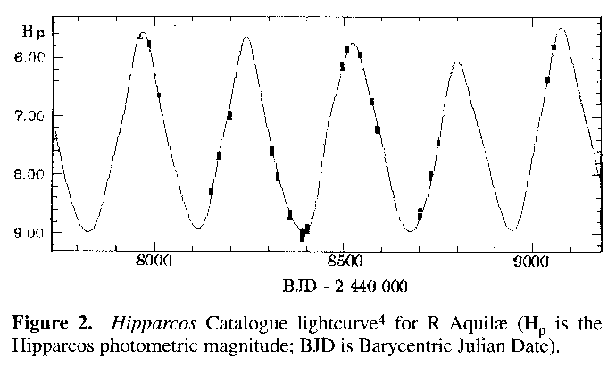
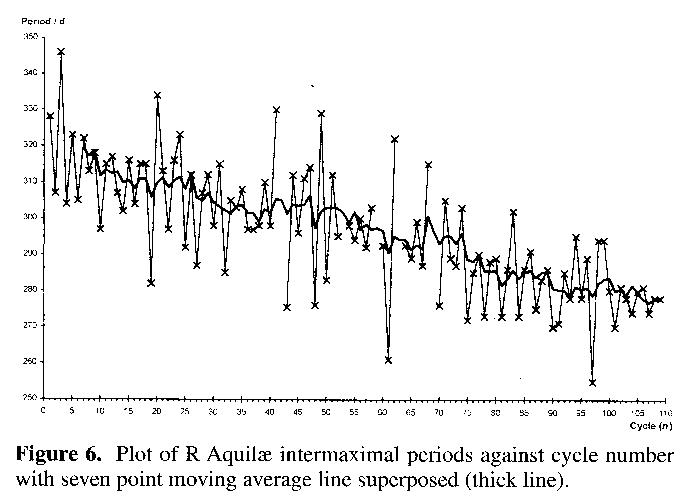
Figure 1 shows the light curve for R Aquilae.17 Figure 6 is a representation of the periods from Table 1, plotted against their cycle number. The individual points are connected by thin lines and a denser seven point moving average line is superposed, the better to illustrate the overall decline in period.11
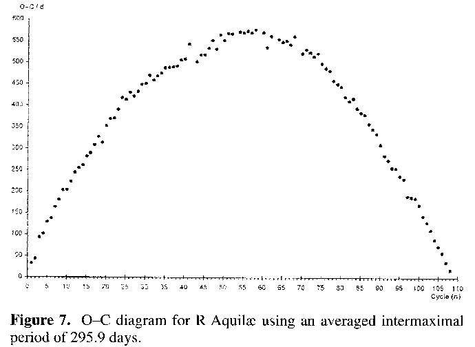
Figure 7 shows the O-C using the test period based on the average intermaximum length of 295.9 days. It can be seen to be a symmetrical curve about the centre of the plot, and suggests that the period was longer in the past compared to this central point and has continued to shorten since then. The quadratic fit of -0.93x2+20.91x (for zero intercept) gives a best fit line with R2 = 0.99. R2 is the coefficient of multiple determination and takes a value between 0 and +1, in the direction of increasing fit. In its use here it takes the positions of the real data in the x-y scatter graph and compares them with the assumed positions on an equivalent best fit line derived from a given formula (the quadratic fit here). In this case the match between the quadratic best fit line and the data rates as 0.99. A typical O-C chart shows no such regularity and considerably more scatter in the data points, as Figure 8, an O-C chart for X Camelopardalis from BAAVSS data shows.16,17 A quadratic best fit line to the X Camelopardalis data has been generated for illustrative purposes: in this instance the best fit line only has R2 = 0.62.
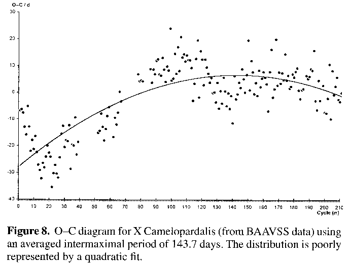
Figure 9 is the power spectrum for R Aquilae from the raw data, over the period range of 250 to 400 days (0.004 to 0.0025 cycles per day). Few if any other significant peak occurs down to periods as short as ten days, save very small harmonics of the main peaks at exactly half their periods. There are two main groups of peaks, the leftmost of which consists of a set with the strongest one being of about 306 days period. The right hand peak attains a maximum at around 282 days. These peaks show that more than one period has existed over the time interval of the data, a point of interest considering the repetitive regularity and overall stability of the visual lightcurve. The expression of many periods in the form of two discrete peaks at either end of the frequency range is most likely due to cancellation of power in the mid ranges caused by interference between peaks at adjacent frequencies.20
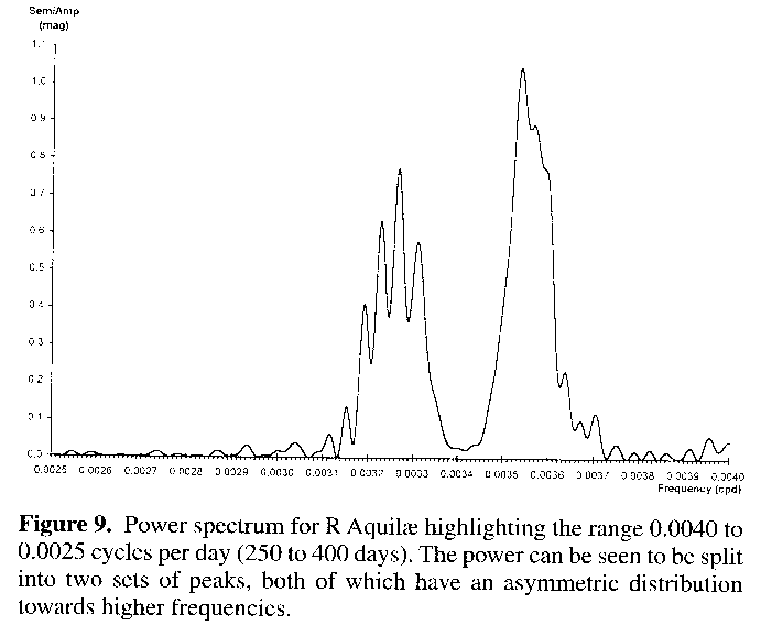
However, interpretations based on the detail in power spectra are not straightforward, and to some extent the fact that it is already known that R Aquilae is declining in period is bound to colour judgement. On the other hand, the fact that the data is on the whole quite complete and continuous allows a certain amount of confidence to be placed in an interpretation of varying period in this instance, Miras not usually possessing contemporaneous adjacent period multiplicity, which would be an alternative conclusion. Such stars do exist, but these are semiregular variables with quite different lightcurves.
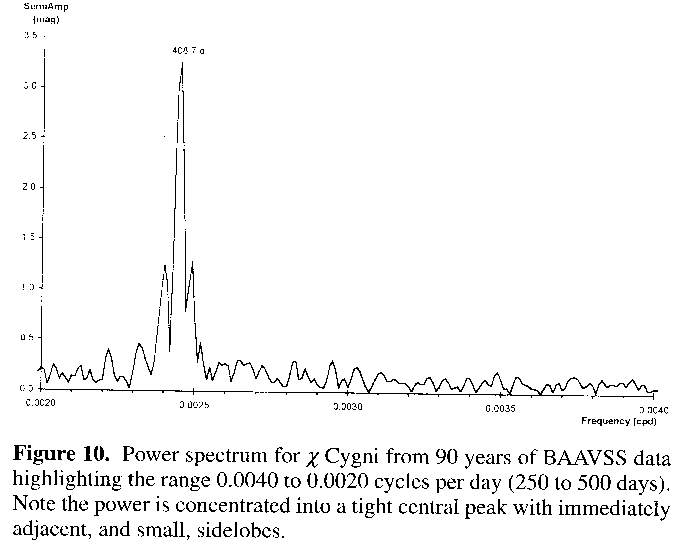
Figure 10 shows the normal situation for Mira star power spectra, here for c Cygni:16 note a narrow main peak with small mostly symmetric sidelobes (although low amplitude peaks due to harmonics do occur at higher frequencies than those shown, which are related to the humps this star often displays on its rising light curve).
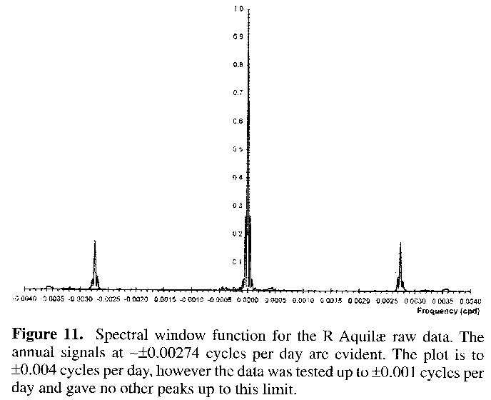
Figure 11 is the spectral window function from the raw data for R Aquilae. The central peak at zero frequency represents the normal situation. Distant peaks extending to either side highlight other periodicities within the time sampling of the data. The most evident peaks are the ones at around +/-0.25 relative amplitude, which are representative of the duration/timescale of the data. The annual signal at around +/-0.00274 cycles per day can also be found, of relative amplitude 0.18. Note that the latter are each accompanied by small side lobes, which represent the beat periods between the annual signal and the positive and negative data timescale peaks. Despite this being only a low resolution scan, there is very little evidence for any other period hidden in the data's structure (although an intriguing pimple of 0.01 magnitudes relative amplitude can be seen at a frequency equivalent to 282 days, possibly coincident with the timescale of observation for binocular observers,21 to whom the star is invisible during times of minima).
Figure 12 is a plot of (inverted) phase and amplitude against Julian date generated via the AMPSCAN methodology, using approximately 5,000 data points generated by taking the 5 day means of the complete and raw data set. A period of 315 days was used, being roughly the average period for the first decade or so of data,2 and the data were calculated upon Nyquistian windows of 10 days. The resultant plot has the phase calibrated by setting the lowest value to zero. It can be instantly seen that the plot of phase against time emulates the O-C plot generated if a test period of 315 days is used, with O-C residual in days replacing (inverted) phase in degrees (Figure 13). Similarly an AMPSCAN (figure not shown) based on the averaged intermaximum period of 295.9 days produces a plot of phase against time that emulates Figure 7.
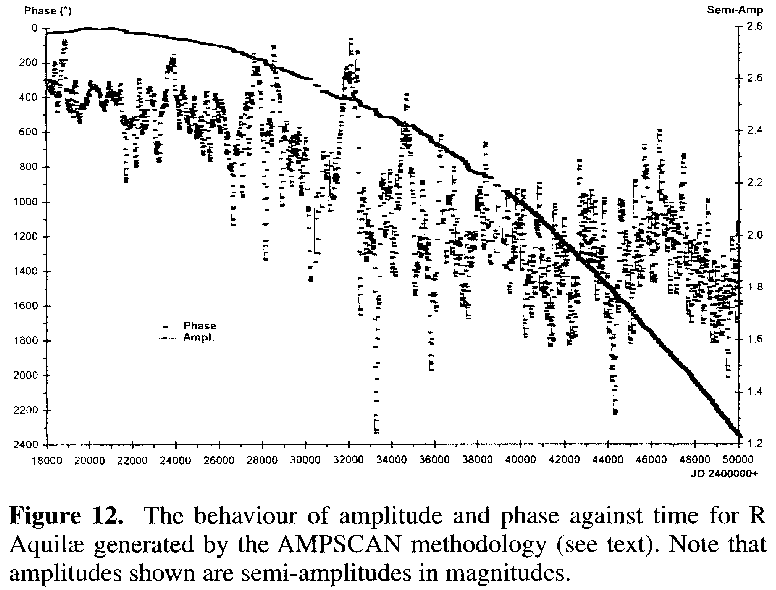
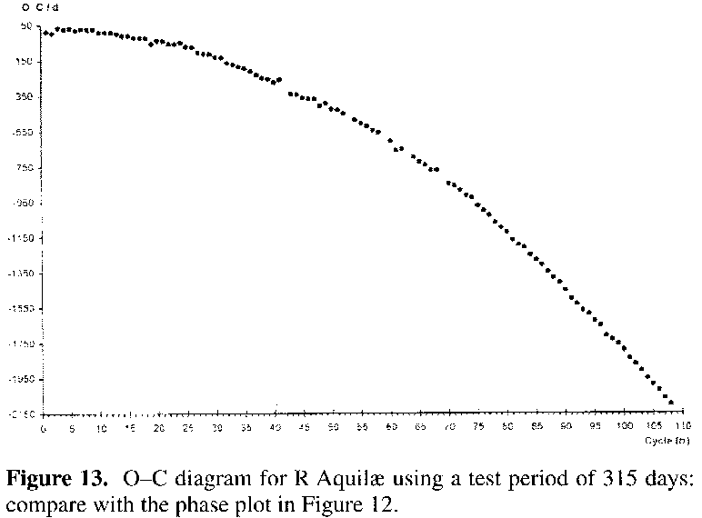
It is usual to use the average period in both the generation of O-C and AMPSCAN plots, and this has been the case for all the stars mentioned here, save R Aquilae. In R Aquilae's case emphasis is placed on the plots derived from the extreme period of 315 days for descriptive purposes: it is easier to illustrate the decline in this way.
All in all phase is occurring at an offset of approximately 2400 degrees by the end of the plot, equivalent to being ~ 6.7 (2400/360) cycles earlier than it should have been given a constant period, in comparison to the situation at the start of the plot. Similarly, the most deviant O-C residual generated by the 315 day test period is ~ -2100 days, again roughly 6.7 cycles (2100/315) 'earlier', as the negative sign suggests, than it should be. The phase against time plot depicts the period shortening better than the O-C plot does, showing even less scatter about the parabolic decline. Further, the phase against time plot samples the entire data set, not just the derived dates of maximum, and in this instance helps to show that the decline in period for R Aquilae has been quite constant throughout. Minor deviations and gaps reflect more the varying density of the data rather than any real event.
The semi-amplitude against time plot also suggests a constant decline, although with not such a good linear fit in this instance. It should be remembered that amplitude is expressed in magnitudes, which is a logarithmic system, and therefore liable to linearize data via scaling effects. Despite this there still appears to be a great deal of scatter in the trend in amplitude, when compared to that of phase. Some of the larger variations will no doubt be due to errors in the process caused by thinness of data from time to time. Some will be real.
Mira stars of spectral type M do not decline in the visual range merely because of radius and effective temperature variations, thence luminosity (and its relative measure, magnitude). Titanium oxide (TiO) condenses out of the atmosphere as it cools, and this material is highly opaque at visible wavelengths, causing dark absorption bands across the spectrum, and thus subduing the total flux in the visual. The relative levels of this condensation from cycle to cycle, plus other not entirely understood mechanisms, superimpose their signature upon the merely pulsational nature of Mira stars, constantly modifying (and frequently hiding) it.
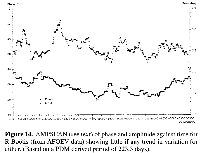
Nevertheless the AMPSCAN methodology clearly demonstrates R Aquilae's fairly regular trend in descent of overall amplitude over time, something that even consecutive maximal magnitudes rarely show up well. Most Mirae show little overall trend when amplitude is plotted against time via the AMPSCAN method, usually having erratic fluctuations towards both increased and decreased amplitude that more or less average out over time, as the plot generated for R Bootis16 from AFOEV data22 for the time interval JD 2440000 to JD 2450000 using a mean period of 223.3 days shows (Figure 14).
As explained in the methodologies section, the phase and the amplitude can be further depicted by compounding them into a two dimensional complex phase space, as shown in Figure 15. Each short horizontal bar represents a value at every ten days, with a thin line connecting to reinforce the feel for the direction of motion. Also, superposed filled circles denoting the time when every nn thousandth Julian day has passed are included, their numeric labels thus representing JD 24nn000.
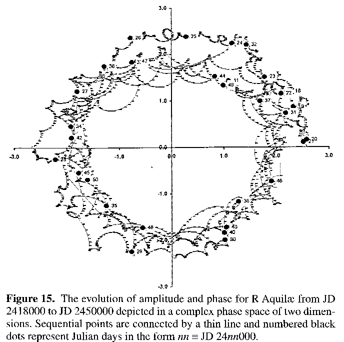
As can be seen, the transverse motion depicted in the plot wanders slightly from JD 2418000 to JD 2421000, after which it begins to follow a strong, rapid and ever increasing anticlockwise dash around phase space as the current average period gets further and further away from the original one of 315 days: the motion adds up to roughly 6.7 complete circuits (compare with other results above). Radial motion in this two dimensional phase space depicts variation in amplitude, and by following the dates superposed on the plot this amplitudinal component can be seen as a helical modification of the transverse motion. That is, the plot increasingly approaches the origin of both axes.
A plot derived from the use of the averaged intermaximum period of 295.9 days is similar, but consists of points that first circle clockwise, then anticlockwise after a brief 'standing' phase at the point when the true period was close to the average period used. Also the amplitude is distributed bimodally about this point, as opposed to helically (figure not shown). In both plots the paths followed are not necessarily simple arcs, but exhibit cusps and occasional loops. These cusps denote points which are harmonic to the period used to generate the original data.
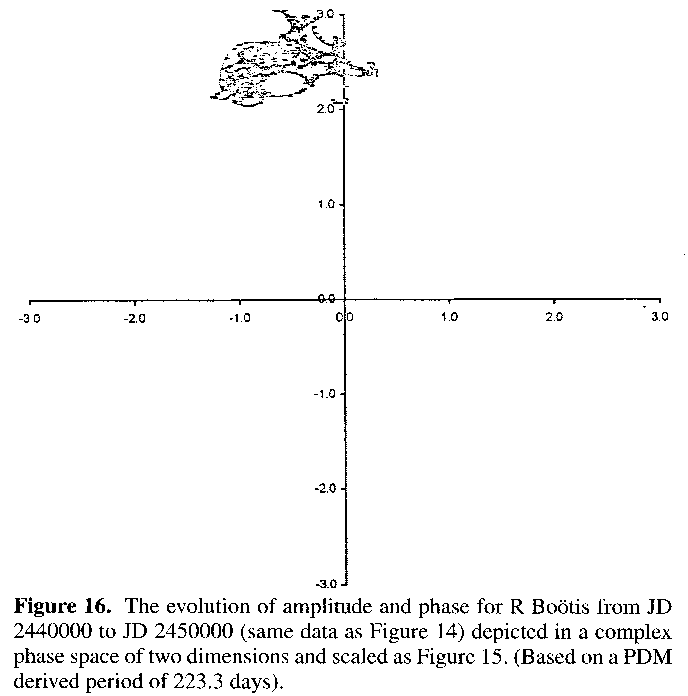
Most Mira stars simply mark time around their average period, as is again well illustrated in Figure 16 by the same data for R Bootis16,22 used in Figure 14, after it is converted into a two dimensional complex phase space. Using the same axis extrema as for R Aquilae we find a good representation of small scale random transverse and radial variation about central core values. This well represents the usual problem with analysing the evolution of period and/or amplitude in Mira stars: the plot looks little different from one that would be expected from scatter in the data. This again reiterates the difficulty in distinguishing trend from temporary random fluctuations and/or observational scatter within visual Mira star observational data sets.
Summary of descriptive investigations
The O-C defines the symmetric parabolic shape expected from use of an averaged test period upon data representing a range of constantly varying period. Plotting the O-C using a test period representative of the first decade of data2 also revealed the decline in period via the decline in O-C residual. That this decline is well regulated and consistent throughout the past ninety years is strongly supported by the good fit which a quadratic expression is capable of giving when placed against the data. Even a plot of periods against cycle number shows a definite declining trend (Figure 6).
The power spectrum revealed evidence for more than one periodicity, centred about two main cores, which may mark the remnant of a broader peak that has undergoing cancellation in the central regions via interference between adjacent periodicities. Conversely, the spectral window function revealed no period inherent in the spacing of the data save that for the timescale of the data set and that for the annual alias, plus beat periods of the two, i.e. a lack of false periodicity signals. R Aquilae's light curve is well represented by a sine wave of one period: hence multiple periodicity depicts variation in that period, and not harmonic and/or other, more complex, contemporaneous periodicities.
The 'new' AMPSCAN methodology illustrates the situation well, the phase (when inversely plotted) mimicking the O-C generated for the same test period so well that it would be more appropriate to say that the latter emulates the former. Extension of the phase and amplitude into a two dimensional complex phase space allows the details to be followed further, showing the combined effects of trends in phase and amplitude upon each other.
In the case of R Aquilae nearly every analytical procedure tells us something about the star's variation in period over time, and sometimes also for that of its amplitude. Examples of other Mira stars given in comparison on occasion have shown that this may not always be the case. However, although these procedures (especially the statistical ones) can show evidence of something happening, they are not geared towards showing that nothing is actually happening. That is, lack of evidence for variation does not mean evidence for lack of variation. Such variation has merely not been found and may still exist, hidden from our view.
It is still often the case that apparently self-evident phenomena gleaned from a cursory visual inspection of a light curve cannot be confirmed by any of these methodologies. Even if the tests do confirm any suspicions, we are still left with the fact that none of these tests can actually be proof of anything, but can at best be merely highly suggestive with regards to patterns in the data. In the case of R Aquilae it would be churlish to suggest that none of these effects are real, but when it comes to other Mira stars the situation is rarely so clear cut.
KL11,12,13 have developed new methods for removing error from the investigations upon Mira periodicity, but these methods are rather beyond the average interested amateur, if not even the average professional, being more suited to the specialist statistician. As of yet neither of the authors know of any application of these methods for use on personal computers. Such would be welcome given the number of Mira stars having a wealth of observational data for them nowadays, often already in a fairly accessible machine readable form.
Indeed, it is about time the emphasis shifted from the archiving of data to its analysis. Visual observations conducted by amateurs over the past century have been strongly biased towards Mira stars, and although it is often very difficult (if not occasionally impossible) to glean anything from these data, due to their observational scatter and the capricious behaviour that these stars exhibit (they often being the most irregular of regular variables), such a treasure trove of data cannot be ignored. If current methods of investigation are inadequate, new ones must be made available.
It is felt that the AMPSCAN method14,15 goes some way towards addressing this problem at least in the descriptive sense, and possibly even via the statistical manipulation of the data it generates. However, it (and other methods, including some of those of KL) is heavily dependent upon complete and dense data sets, and it is now time that some of the more possessive aspects of data archiving were relaxed.
The hard work of observers both past and present should be fully acknowledged, as should that of the organisations that collect, collate and archive the data in a form suitable for use. But when the fact that few data sets are complete for any particular star is combined with the fact that very few long period variables actually present any evident behaviour worthy of fuller investigation,16 as well as the unfortunate reality of the two subsets rarely overlapping, then every little bit of available data is priceless.
WZ also mention R Hydrae as a Mira star classically known to be declining in period. Unfortunately the data for this seasonal and southern star are somewhat thin and patchy, such that it is very difficult to be sure what the results are saying. It does appear, however, that the decline for R Hydrae16 is not as regular as that for R Aquilae, so it may not be a helpful comparison object after all: indeed if data existed for this star from only JD 2432000 onwards, they would show little or no sign for period variation.16
Data from various sources for about 100 Mira stars were examined in the hope of finding another star similar in behaviour to R Aquilae, a process facilitated by the utility of the AMPSCAN procedure which enables relatively quick and easy processing in comparison to more traditional methods. Firm evidence could only be found for one such star, specifically the star T Ursae Minoris as represented by AFOEV data.22 On alerting AFOEV of this fact JG was not surprised to be informed that this star and its behaviour had already been well examined,24 on at least two separate occasions.25,26
T Ursae Minoris began a constant decline in period at around JD 2445000 (early 1980s), moreover the decline on an O-C plot can be fitted by a quadratic expression with an R2 equal to 0.999.16 Prior to this decline T Ursae Minoris erratically varied in period (in the usual Mira-esque manner) about a roughly 315 day average, which is not an uncharacteristic value for a Mira star. Nowadays the average period is not much different from that of R Aquilae (between 270 and 280 days), so that in the space of barely twenty years T Ursae Minoris has managed to achieve the same extent of period decline as it took R Aquilae 90 years to do, and just as cleanly too. Interestingly, T Ursae Minoris also gives evidence for a declining semi-amplitude since ~ JD 2445000, with a linear trend16 of the same order to that for R Aquilae (average rates of 3.4 X 10⁻⁵ and 2.6 X 10⁻⁵ per ten day sample, respectively), although it is still too early for that of the former to be reliably determined.
Finally with regard to period decline, Gunther24 notes that there is growing evidence for the dominant pulsation mode of Mira stars being in the first overtone (first harmonic) for objects with periods in the range of 280 to 430 days. Both R Aquilae and T Ursae Minoris are approaching, if not rapidly surpassing, this theoretical lower limit. Does this mean that some dramatic variation in the periodicity of these stars will occur in the next decade or so? As usual, we can only wait and see.
Period-luminosity laws have recently been defined for long period variables (LPVs) utilising K band (l = 2.2mm) photometry, specifically the mean magnitude at this wavelength. This ultimately involves calibration against groups of LPVs at known distances, for example in the stellar association Perseus OB1 or the Large Magellanic Cloud, so that the absolute magnitudes in the K band can be derived for objects of known period. Subsequently stars of known period and known mean apparent K band magnitude can have their distances determined via derivation of their distance moduli (i.e. difference in apparent and absolute mean magnitudes in the K band).
The K band is however an infrared band that is not directly amenable to amateur observation. The AMPSCAN methodology almost uniquely permits the derivation of a mean amplitude over a set timescale to a fair degree of accuracy, which in combination with derived periods may also reveal an amplitude-period relationship for Miras, given a statistically adequate number of objects with known data. However, scatter in amplitude at visual wavelengths due to the effects of TiO absorption may still prove too problematic.
R Aquilae is a special case where the presumed physically driven decline in period and amplitude over time is of sufficient scale and consistency to override the usual scatter, thus providing a statistical sample of periods and amplitudes taken over time with respect to the one star, as opposed to the usual case of contemporaneous snapshots taken for many differing stars. In Figure 17 the AMPSCAN results were used to derive average amplitudes about timespans of a thousand days duration starting at JD 2418000. The maxima derived for R Aquilae were then used to give average periods over these thousand-day intervals (each average period being the average of two to four intermaxima intervals).
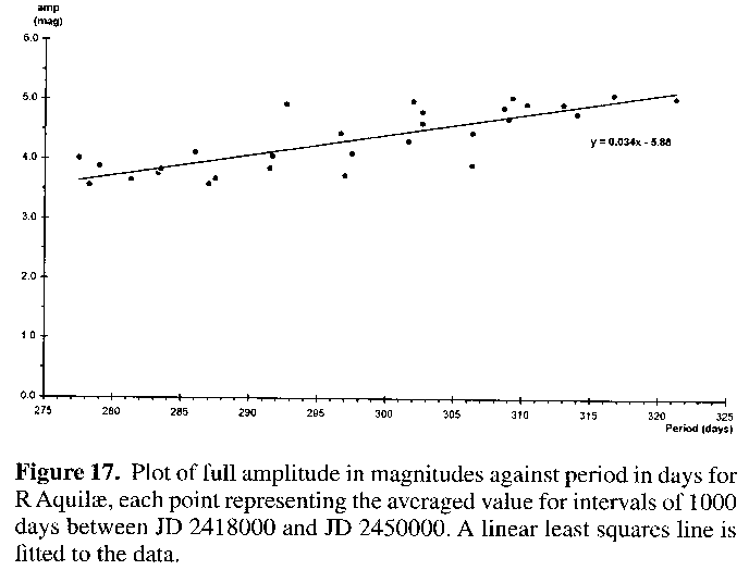
Although the resultant plot suffers from some scatter, a linear relationship of amplitude =0.034 X period - 5.88 fits the data quite well, a fair result considering the simplistic approach used for this preliminary investigation. Hipparcos4 trigonometry suggests that R Aquilae is close enough for a concentrated effort on deriving its true parallax, and therefore distance, to give good results. Should this be the case, then this star could be used to help calibrate any such relation between period and average amplitude (with the more distant T Ursae Minoris possibly being a good check object).
Mira stars are best investigated by a suite of analytical techniques to both reinforce any meaningful results provided by any one technique and also to provide differing aspects/facets of the data. Statistical techniques are useful for removing the subjective nature from any perceived effect or trend, but they are not conclusive on their own and the results therefrom are heavily dependent on the sort of question being asked. They should be used as part of an increasing mass of evidence, preferably including other, independent, statistical avenues.
The onset of remarkably powerful and fast personal computers over the past few years makes it essential that data archives and software applications are made more widely available. There is a great deal of data 'lying around' that is in need of being investigated, if only preliminarily as a means of sorting the wheat from the chaff such that the professional observers and theorists know where to concentrate their attentions and equipment. However, any software made available in the public domain should not only carry good documentation with respect to its use, but also with respect to its misuse, including strong warnings and caveats with regards to conclusion jumping and the need for rigorous adherence to basic analytical procedure.
Both authors would also like to strongly acknowledge the contributions of all the observers, both dead and still living, without whom this article would not have been possible. Both the authors have done their share of making visual estimates of variable stars in the past, and realise the amount of effort it involves. Hopefully this article goes at least some way towards thanking these people for their efforts.
Many of the periodicals referenced in this article were sourced via NASA's Astrophysical Data System article service: http://adswww.harvard.edu/.
Data for some of the Mira stars alluded to were obtained via the AFOEV ftp site at the CDS, Strasbourg: ftp://cds.u-strasbg.fr/afoev/, and the authors acknowledge the work of the contributing observers and staff of that organisation.