from VSSC97

Concepts of Filtered Photometry - part 1

Graham Salmon

Introduction

The enormous amount of data built up by the traditional method of visual photometry demonstrates that this is an effective method of measuring the light output of a variable star. However, like every system, it has its limitations, particularly in the accuracy which can be achieved (even with the most skilled observer) and the lack of any reference to a change of colour index.

The Light Output of a Star

We are all familiar with the way an object, when heated, passes through the stages of dull red, then cherry red to white hot. Our eyes are only sensitive to a very small part of the whole electro-magnetic spectrum and, even with a large telescope, they are barely sensitive to colour at the very low levels at which they operate with stars.

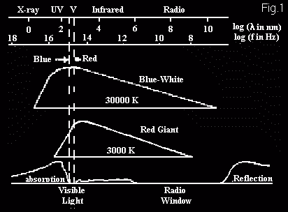
If the complete spectrum of a body at a temperature of 30,000K is measured and plotted, a curve is produced as in Fig.1 which stretches all the way from X-rays to radio waves. It reaches a peak at a frequency of 5x1015 Hz, drops sharply at higher frequencies and much more gently at lower ones.

The output across the visual band from red to blue is a very small part of the whole but is almost level, so we call it 'white hot'. The curve for a body at 3000K, the temperature of a red giant, is also shown. The shape of the curve remains more or less the same, but the peak frequency is proportional to the temperature. This is Wien's displacement law.
Therefore, if we want to know the temperature of a star, we need to plot its output across the spectrum.
We would use a collimator, slit, prism and CCD to measure the light collected at each point of the spectrum. However, this would spread the light over a large area and would require a much longer exposure for the star. This would severely limit the stars attempted to brighter ones.

Colour Indices

We do not need such detail. We can have a measure of the general shape of the spectrum of a star by sampling it using 'broad band' filters. The spectrum from the UV to the IR can be divided into five under a system known as Kron-Cousins, and ideally each filter would have a similar transmission characteristic as shown in Fig 2.

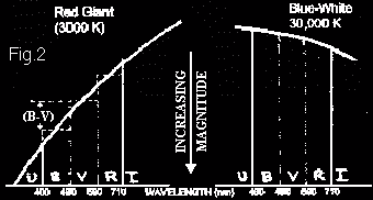
For each star, the difference between the adjacent bands (B-V), (V-R) etc., will provide a measure of the slope of the curve over that part of the spectrum, and hence an indication of the colour balance and temperature.
These are called the Colour Indices. (B-V), the most commonly quoted parameter, ranges in main sequence stars from -0.4 for a blue-white star to >1.5 for a red giant. (As magnitudes increase as the star is fainter, these values go in the opposite direction to first expectations!) The 'colour temperature' derived in this way is that which a 'black body' (or perfect radiator) would have with this colour index. However, it should be remembered that the constituent elements and physical processes in the star will distort the pattern of radiation, so it will be somewhat different from the effective temperature. However, 'colour temperature' is still a useful concept.

A Filter System

The CCD has the useful characteristic that the charge generated in each pixel is closely proportional to the light falling on it. The software supplied with CCDs usually has a facility for measuring this. The CCD also enables simultaneous observation of the variable and comparison stars which come within its field of view (which is not the case with photomultiplier tubes).
As most of us have to be content with one telescope and one CCD, the four or five filters on it need to be mounted so that they can be changed easily, ie. on a rotary or slide carrier, and the method of measurement has to take account of the fact that the exposures are then taken in succession rather than simultaneously, so that the sky conditions may well have changed from one frame to the next.

The frames will show the variable (V) and comparison stars (1,2,3 etc) some of which will be brighter in the blue and UV, and others brighter in the red and IR. After pre-processing, suitable software can measure the brightness of the variable and each comparison star on each frame (U, B, V, R and I), and express it as a magnitude.
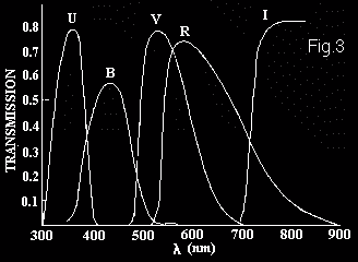
Actual filters are made of coloured glass and have a response as in Fig.3 - peaking at some central frequency and dying away on each side, overlapping into the area of the adjacent filter. To complicate matters further, the CCD also varies in its response as in Fig.4, with substantial differences between different types of CCD.

So the magnitude read by the computer off the CCD frame will depend on the intrinsic brightness and colour index of the star, the sky conditions, the telescope and filter, and the CCD. Before proper observations can begin, the system has to be calibrated.

Callibration

We require a set of factors known as Transfer Coefficients, which we can apply to actual observations to correct for the characteristics of the system.
To determine these factors, we need to use a group of standard stars which vary in colour index, but can all be included on one frame and whose UBVRI magnitudes have been carefully measured. The group most frequently used is in the open cluster M67 and consists of eight stars ranging from red to blue-white. Exposures are taken through each filter in turn, and then, after pre-processing, the photometry is done on each frame and the results are recorded.

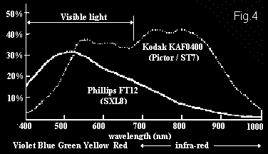
There are two types of coefficient:-

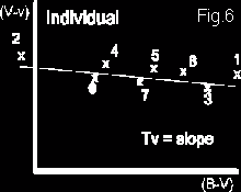
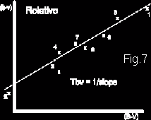
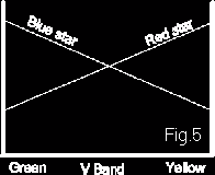
a. For each individual filter - a factor is required which relates the way the sensitivity of the system varies with the colour index of the star, ie. if, as in Fig.5, two stars have the same total output between green and yellow, but differently distributed, how does the instrumental magnitude vary? For each frame, the difference between the standard and instrumental magnitudes of each of the eight stars is plotted against their respective colour index as in Fig.6, and the best fitting slope determined. These Transformation Coefficients are known as tu, tb, tv, tr and ti. The slope should be around '0', ie. the the instrumental magnitude relative to its standard value should not change much, if at all, with colour index.

b. For each pair of adjacent filters - a factor is required which relates the way the relative sensitivity varies with colour index of the star.
For each frame, the instrumental colour index of each of the eight stars is plotted against their respective standard colour index as in Fig.7, and the best fitting slope determined.
The Transformation Coefficients are the inverse of these slopes and are known as tub, tbv, tvr and tri. Their value should be around '1', but will probably be somewhat greater, ie. the sensitivity when using the B filter is less than when using the V filter (mostly due to the CCD) so that subsequently, when using the system for actual measurement, b values will have to be increased by say 1.5 to get the true values.

In practice, only some of these coefficients are required, depending on circumstances. For instance, if one was only using the B, V and R filters, the V measurements would form the base and require the tv coefficient, while the B and R measurements would be made relative to this and just require the coefficients tbv and tvr.

Extinction Coefficients

These must be mentioned, if not elaborated upon, at this stage. As we all know, the sun is redder when rising and setting because of the greater depth of atmosphere through which the light passes compared to when it is overhead. This means that the atmosphere absorbs much more blue light than red. The same thing happens to starlight even though this is not noticeable to the naked eye. Therefore, when making observations for photometric purposes, the altitude must be noted and an Extinction Coefficient applied to allow for this. When applied it corrects the magnitude to the value it would have if the observation had been made above the atmosphere.

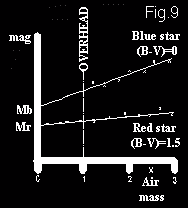
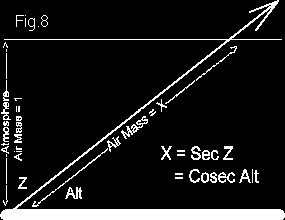
Fig.8 shows this for a flat earth which is acceptable for us as long as the altitude of the star is >30°. The depth of the atmosphere through which the light must pass is called the Air Mass and, relative to the distance when it is overhead, is equal to Sec Z, the zenith angle, or Cosec Alt.

If a close pair of stars, one red and one blue, is observed rising from near the horizon to the meridian, their magnitudes determined and corrected with the transfer coefficients, and then plotted against their respective air mass as in Fig.9, two lines will be produced, one for the red star and one for the blue. These can be extrapolated to the vertical axis to derive the magnitudes that would have been measured if it had been done above the atmosphere. The extinction coefficients can be derived from this.

Conclusion

The principle object of this whole exercise is to provide our professional colleagues with high quality data, to an order of accuracy of 0.01 magnitude, and to be able to apply this to rapid changes say in the outburst of a cataclysmic variable. This will enable them to do a more thorough analysis of what is going on. A successful outcome will depend on many factors - the equipment available and skill in handling it, the care in processing and photometry on the computer, and the reduction of the data thus obtained.
I hope to be able to go into more practical details in future issues.