This is a summary of the following meeting. An edited version of this report will appear in the BAA Journal, and in VSSC number 110. The whole meeting was recorded on video; the six videos are available for loan for the price of the return postage – please contact the Variable Star Section director for further information.

This year BAA members were given a real treat, in the form of a weekend meeting of the Variable Star Section, held at Alston Hall in Preston. This was ably organised by Denis Buczynski and Roger Pickard, and got off to a lively start on the Friday evening, with Dr Allan Chapman's talk on 'A History of Variable Star Astronomy.

Halley was also the first person to write seriously about variable stars and nebulae, when he published a pair of papers. The first paper was an account of six lucid spots (nebulae) and he pondered what they were and how they might relate to stars; he wondered if they might be densely packed stars. The second paper, published in 1716, was an account of several new stars. Halley was also very interested in what people had seen before him. He brought to astronomy, the idea that stars might have changed in some way over recorded history. He believed that there were two classes of variable stars. One class included supernovae, which blazed up and then vanished; he wondered what they were, and how they related to other stars. The second group were stars that changed in brightness and colour - mira type stars (mira means wonderful in Latin). Halley wondered why these stars were variable. So it was Halley who effectively established variable star astronomy, and he also provided theories as to why the stars should change.

It intrigued Halley why the sky should go dark at night, as he believed that there must be a star wherever you look (dark matter was not known about at this time). He argued that stars are point sources, and point sources take up no space, so they must be surrounded by a dark annulus which is bigger than the star itself.

Another astronomer who contributed greatly to variable star astronomy of the time, was John Goodricke. He was born in York, a deaf mute and a brilliant mathematician, who died at the early age of 22. He started using a friend's 3.75 inch Dolland refractor to observe, together with a good quality regulator clock, which allowed him to measure to within tenths of a second. He started measuring the eclipsing binary Algol, making photometric estimates of its brightness. In 1782, he derived an orbital cycle for Algol, that is to within a minute or two of current day measurements. Two years later in 1784 he published a paper on Delta Cepheus, in which he reported his measured period of 5 days, 8 hours and 37 minutes. He noticed that the Delta Cephei and Algol light curves were very different to one another.

It was Daniel Huber who first suggested that Goodricke’s light curve might be evidence of a binary system. There was great interest in binaries at this time. Herschel was also interested in Algol; he thought that if Algol was a geniune binary, then you should be able to see the binary using an eclipsing bar. He tried this, but he could not see it, so the speculation remained.

Friedrich Argelander started to try to get astronomers to search for variables, in the mid 19^th century. He pointed out that this kind of work was ideal for amateurs, and he suggested that a kind of international police be set up, to look for stars that changed in brightness and also in colour.

In 1782 Herschel published his first list of double stars, which was later expanded. By 1802, it was noted that some of these binaries had changed their position relative to each other. At this time 'variable' meant something that changed, and so included binaries. Bessel and John Herschel asked whether these stars were conforming to Newtonian criteria, if they were moving in relation to each other? The stars were well studied, and Herschel and Savary made the first analyses of their movements, and discovered that at least one of these stars had elements that suggested that they did satisfy Newtonian gravitational relationships.

By 1840, numerous astronomers were measuring variable stars. This took a long time for many stars, and could only be done by professionals with big telescopes, or rich amateurs. In the1830s, Bessel suggested that those stars with the greatest proper motions might be the nearest to Earth. So if you could find a binary pair that had a big proper motion, then you might be able to measure them more easily; this provided a selelction criterion. With this increasing amount of data, Bessel noticed the wobble of Sirius, and in 1844, he suggested that Sirius might have a dark companion. This was discovered by Alvin Clark in Boston in 1861, by using an obscuring bar, in conjunction with a large refractor.

By 1840 lots of variable stars were known. It was in 1834 that John Herschel arrived in South Africa. Watching the stars from the ship on the journey, he learnt his way around the southern sky. He questioned if the stars were the same brightness, and went on to invent a technique for measuring the relative brightnesses of these stars. He put the moon on the horizon, and devised a way of shutting down the moon's light until it was exactly the same brightness as a first magnitude star. He then calculated that a first magnitude star was the same brightness as a certain fraction of the moon's diameter; it gave him a standard to measure the brightness of stars by; in this way Herschel did some of the first work in comparative photometry and others went on to develop the technique further.

Once glass making techniques improved, Pritchard invented the graduated wedge. This comprised a wedge of glass, which was dyed uniformly throughout. The wedge was then used to see where along the glass, the star's light first disapppears.

By the 1900s, the concept of photographic magnitude was begining to be developed, after Pickering started to develop the first nomenclature for stellar brightness. The spectroscope was also being developed; Vogel pointed a spectroscope at Algol and noted that the spectrum was split; he was able to note the composition of the stars, the relative masses of the stars, and the size of the orbit.

By the 1840s astronomers knew that the sun's light output was not constant. Geologists' studies of rocks suggested that the earth's climate had changed a lot, and astronomers speculated that it probably had something to do with the sun. Louis Agassi studied the way glaciers had carved trenches out of the land, and William Buckland wondered if Scotland had also been covered with glaciers. They surmised that the sun must have a variable cycle. Heinrich Schvabe was a postman, who observed sunspots, and began to notice a cycle. He wrote a letter to Alexander von Humboldt about this, and Humboldt mentioned the postmaster's observations in Kosmos.

In 1865 ,the first spectral classification was published by Secchi, and by 1880 it was thought that all stars might be variable given enough time. By this time there were several big observatories being built, such as Stanford and Yerkes, with enough funding to pay staff. Harvard realised that they needed better skies, so they aquired a site in Peru and started systematically photographing the skies, and sending the photographs back. Women back at Harvard worked on plate measuring machines, and made delicate photometric measurements; searching for anything that changed. It was noticed that in the SMC there were a number of variables, and that some had the same light output pattern as Delta Cephei. Henrietta Leavitt noticed a pattern between the brightnesses and the period of the light curves, and suggested that there might be a relationship between the period and the absolute brightness of the stars; this would give a method for calculating the distance to a star. Shapley started to do an analysis of 11 cepheids with known pronounced proper motions, but there still remained the question of how you relate these to other cepheids that are further away.

In 1885, a supernova went off in M31. By this stage astronomers were just able to make photometric brightness measurements, and found that the supernova was giving out one tenth the light of the whole galaxy. This lead them to the false assumption that the galaxy couldn't be too far away. In 1924, a cepheid, was found in the same galaxy, by Hubble using the 100 inch telescope, and he managed to use Leavitt's relation to get a true idea of the distance to the cepheid. Variable stars have been at the heart of our attempts to discover what the universe is like.

What's the mechanism that operates within a cepheid? It was explained the pulsation of the cepheid was maintained due of the ionization of hydrogen, a theory which probably came originally from Eddington.

Gary Poyner asked Dr Chapman if he would speak about John Russel Hind, who discovered U Gem. Dr Chapman said that Hind was a son of a lace manufacturer, who worked at observatories before working for the Nautical Almanac. He left school at 17, and later made major discoveries. It seemed like he never felt truly part of the astronomical community, as in 1851 he was elected a fellow of the Royal Society but did not turn up to sign the book, which was a requirement of receiving the award. Later, when he was elected for a second time, he did turn up to sign the book. He was an observer of variables and binaries.

Nick James asked when light curves were first produced. Dr Chapman said that probably Vogel and especially Shapley after 1910, popularised the technique. Dr Chapman added that in 1801, William Herschel (the father) noticed changes in the number of sunspots, and asked if they were indicative of the sun’s variable energy output? He noticed that when they had a few good years of weather and good harvests, that the price of bread would drop; he then analysed the price of bread over a period of time and found a periodicity! This was probably the first time that a scientific connection had been realised between changes in an astronomical body and terrestrial ecology.

Space had been made in a separate room to allow for members to exhibit posters showing their work, and at this session, these members were invited to make short presentations introducing their work.

Melvyn Taylor began the session by discussing his attempts to follow WZ Sag in outburst, visually, and showed his light curves. He also showed the binocular priority list that is produced, and said that he felt that the list should be updated. He thought that this should be discussed on Sunday, as he did not want to exclude any stars that people felt should be left on the list.

Graham Salmon discussed the clear sky detector that Richard Miles had presented at a meeting some time ago, and described how he was inspired to make one. Now he is able to sit in front of his television, and be alerted by a buzzer if the sky becomes sufficiently clear to observe! He also mentioned Norman Walker's filter box which he uses for photometry, and how he modified it to allow it to be driven by a stepper motor, so that the filters can be changed automatically.

Tom Lloyd Evans has recently moved back here from South Africa where he worked for many years at the South African Observatory. He was aware that some of the South African telescopes do not have their time fully allocated, and he wondered whether there might be the possibility of sending out experienced observers to do work to extend chart sequences using some of this surplus time.

Denis Buczynski mentioned his poster which describes his work to develop equipment that will produce measurements, that will be useful to other people. Nick James has developed software for Denis's 13" automatic telescope, which means that Denis can sit in front of the television, whilst observing. Denis is also building a new robotic telescope in conjunction with local universities, which will use parts of a 24" telescope that Gordon Bromage has offered on a long term loan. It is hoped that it will see first light this time next year. This telescope is being constructed with an altazimuth design which may prove challenging!

Roger Pickard mentioned the Jack Ells automatic photoelectric telescope, which was built around 1988. After Jack's death, it was moved to Malcolm Gough's house for use. It was fully automatic, and could be set up and left. It didn't even matter if it rained as it was designed to be able to withstand getting wet. Although the telescope still worked well, Roger suspected that photometrically the weather had deteriorated over the last few years.

Roger Pickard mentioned that Dave McAdam, had had to step down as computer secretary, but that John Saxton had now taken over, and Peter Moreton was the new Variable Star Section Web Master. The BAA had decided to move to a new web provider (their new web page address was http://www.britastro.org), and so the Variable Star section had also moved their web page; the new address was http://www.britastro.org/vssc.

Norman Walker asked, and Gary Poyner agreed that there should be a standard format for the reporting of observations, as people had been sending in WZ Sge observations in in many different formats. Roger said that all the professionals usually wanted was magnitude or delta magnitude and Julian Date. Karen Holland mentioned that she felt that many professionals would also require error bars.

Albert began by describing the properties of miras: they generally had periods of 200-600 days; visual amplitudes of >2.5 magnitudes; the periods were stable, but the amplitude could vary, and they had strong stellar winds. Semi-regular variables, on the other hand, were very much like miras, but had short periods of 50-100 days; amplitudes of <2.5 magnitudes (SRas had regular light curves, SRbs had irregular light curves) and they all had weaker winds. Albert was particularly interested in how miras changed with time. He showed a Hubble image of NGC7027, and showed that you could just about pick out rings around the planetary nebula. These rings showed that the wind of the mira, which formed the planetary nebula, must have changed with time.

In reality, Albert said, the part of the Mira definition that stated that miras had stable periods was wrong. Some miras showed small variations of about 1-2%, but some changed by much larger amounts. R Aql was discovered in 1850, and by 1900, it was noticed that its period was slowly decreasing. If all the exisiting data was used, the period appeared to have changed from 360 days to around 275 days. The period was due to a sound wave that traveled through a star; if the sound wave took less time to get out (i.e. the period decreased), then it must be because the radius was decreasing. T UMi showed a period of 310 days until 1980, then suddenly the period changed dramatically to 240 days - the star must have changed its radius completely. It was also no longer as large an amplitude variable as it used to be. BH Cru was discovered in 1965, and its period appeared to be rapidly increasing. Its mira pulsations were getting stronger. Apart from these long-term changes (decades to centuries), some stars also showed a cyclical variation in their periods.

R Hya was the third brightest mira at 5th magnitude, and had a period of around 400 days. Its period evolution, discovered in the 19^th century, was described in 1981 by Wood and Zarro. There appeared to have been a continuous decline in the period since at least 1850. Since 1950, the period had been constant at 385 days. To detect the start of the decline required historical data, and Albert had found records of all the observations of maxima since 1850, and records of older observations dating back to 1662. It looked like the period was constant many years ago, and that the period started declining around 1770 (to around 400 now, from 500 in the 1700s). He also had IRAS data which showed the dust shell around the star. It seemed to have had episodes of wind and no wind, and it also looked like when R Hya's period started to drop, its wind ceased at the same time. We know that the wind must have varied with the period changes, and if the behaviour of R Hya was periodic then perhaps the star could blow multiple rings. The rings that were seen around planetary nebulae suggested that changes in behaviour might take place every 200-400 years. Albert had tried to model this behaviour.

In summary, perhaps 10% of bright miras had period variations larger than 5%. They had fluctuating periods; sudden, rapid changes over decades, and slow, continuous changes over hundreds of years. Miras were obviously not quite as stable as previously assumed, so it was important to keep on observing them for a few more centuries!

So what caused these changes? There seemed to be two possibilities. The first was that the helium 'ash' which formed in these stars (due to the burning of hydrogen) might ignite. This could cause rapid changes in the star. The second was that miras might resemble so-called 'non-linear' pulsators, where the pulsation itself caused a change in the star.

Richard Miles asked if big, short term (hours to days) variations at the red end of the spectrum had been observed. Albert said that this was a controversial topic, and that such variations had only possibly been seen in stars of M type not C type. There was a way that this phenomena might be possible, and this involved the sudden formation of TiO in the atmosphere. There was definitely an opportunity here for observers to go out and observe intensely over one night. John Howarth mentioned that in a past examination of Hewitt archive plates, he had discovered a plate on which T Cas was much brighter than it had been observed visually within one night. Albert felt that some caution needed to be exercised when comparing visual observations with photographic observations, as miras were very red, and you needed to be sure that the same filter had been used on both occasions. Gary Poyner mentioned that you occasionally saw hiccoughs on the light curves as they descended and ascended. Albert said that this was a bright 'bump' on the light curve, which was caused by a shock wave, as the inner parts of the star caught up with, and pushed out the outer parts of the star. Tom LLoyd Evans noted that carbon miras show dips at long intervals which are related to dust formation; he wondered if this might be related to ring formation. Albert said that this might be a similar effect, but that you'd really want the dips to last a bit longer to be able to form rings.

Keith started off in astronomy as a visual observer, but because he was keen to do some analysis, he approached Dr Mike Bode asking if he might be able to study for a higher degree, in analysis of variable star data.

Keith explained that a canonical model for symbiotic stars did not exist, only what might be called the 'symbiotic phenomenon', which is most apparent in the spectra of many symbiotic stars. The 'canonical spectrum' (see eg. Kenyon 1986) showed lots of absorbtion bands due to TiO etc., ie. features which are typical of a late type giant in the system. A weak blue continuum was also often present, which was probably caused by a hot star in the system. Finally, pronounced emission lines indicated the presence of a hot ionizing source such as the hot star mentioned above. In fact, some of these lines showed high degrees of ionization eg. HeII and (in one extreme case) FeXIV - the line due to emission by iron atoms with 13 electrons removed. It was the emission lines that Mike was interested in examining in detail.

Symbiotic stars exhibited a kind of double identity, in which they showed semiregular/mira type activity, with occasional dwarf novae type outbursts. Echelle spectra (spectra that were spread out to give high resolution), provided a lot of information about these stars. A survey carried out by a team using the European Southern Observatory and Mike Bode's Manchester-based team, using the Isaac Newton Telescope, produced high resolution spectra of about eighty stars in both the Northern and Southern hemispheres (van Winkel etal., 1993, Ivison etal., 1994).

Both survey teams produced, for each star, spectra of three emission lines (for some stars, several spectra were obtained at various orbital epochs): the H alpha line; the HeII l 4686 line, which is indicative of a hot ionizing source; and the forbidden [OIII] l 5002 line, which is a collisionally excited line, and suggested the existence of an outer low density gas shell, or several outer shells which came about through various outburst phases.

The spectra (most of which were uncallibrated), were produced as plots of intensity vs wavelength, to give the line profile. The [OIII] lines often displayed a very complicated structure which suggested several velocity regimes, and was possibly indicative of earlier outburst phases for the stars concerned (Fig. 1). The HeII lines were invariably single peaked (Fig.2), and relatively narrow; these should have been generated near to the hot source. The H alpha line was single peaked and narrow in some cases, but in most cases it was very broad and double peaked. The blue peak was usually lower in amplitude than the red peak (Fig. 3), but not always. CH Cyg showed the reverse effect, in which the blue peak was higher than the red peak.

Mike had seen such line profiles before in cataclysmic variable star spectra, in which it was universally accepted that double-peaked balmer lines originated from the accretion disc which surrounded the white dwarf star in these systems. He suggested modelling the H alpha lines, on the assumption that they originated in an accretion disc, even though there was still a lot of doubt as to whether accretion discs existed in symbiotic systems. Keith's analysis thus took the form of an investigation, and a single piece of work such as this, could not be expected to prove or disprove the theory at this time. This was a way of approaching the modelling of the line profiles in the most sensible manner. Mike thought that if symbiotic stars did have accretion discs, then it might be possible to have a cataclysmic variable-like system, in which a red giant replaced the red dwarf.

Symbiotic spectra, which displayed narrow single-peaked H alpha lines, could be reproduced by considering the system as comprising a hot star, which ionised a smaller or greater portion of the outflowing low velocity wind of the red giant, depending on factors such as the ionising strength of the hot star, the mass loss rate from the red giant etc.

This kind of model might also explain the presence of the HeII lines in the spectrum, but there was still a problem with the double-peaked lines with their broad wings and central reversal (the dip in the spectral line).

Double-peaked lines were produced by an accretion disc, primarily as a consequence of the orbital motion of the disc material. This resulted in both blue and red Doppler-shifted emission components, which gave rise to the emission peaks, together with a lesser emission component, which resulted from disc material crossing the observer's line of sight (the central reversal), combined with the geometrical pattern of emission from the disc surface. This was illustrated by Fig. 4 which showed the characteristic dipole field pattern, produced by loci of constant radial velocity on the revolving disc surface, and also how the varying lengths of these loci gave rise to different parts of the resulting emission line profile. A high inclination system, ie. one where the disc was seen more nearly edge on, would produce the deepest central reversals. Conversely, a disc seen face on would produce a narrow single peaked emission line.

Early models which were developed to simulate these double-peaked lines, assumed that the disc material was both geometrically and optically thin, ie. emission line photons could escape freely from the disc surface. Observational evidence suggested however, that for cataclysmic variables the disc thickness should be taken into account, and also the disc material was optically thick, ie. some emission line photons would be selectively reabsorbed by the disc material.

Horne and Marsh (1986) developed a new profile model which took these features into account. Their model was able to produce more realistic looking model line profiles. The strength of the Balmer lines in symbiotic spectra suggested that any supposed accretion disc in the system would also be both geometrically and optically thick. Keith consequently adopted the Horne & Marsh model for his investigation into symbiotic stars.

It was time to model real spectra, and to use key features in them (eg emission peak wavelengths, profile wing limits etc.) as anchor points for the model profile fits. Some technical difficulties were experienced in modelling the spectra, mainly due to the quality of the observational data itself (ie. an image intensifier had been used for the observations where a CCD would have been better). These difficulties were eventually overcome using various data analysis techniques and several of the statistical functions in Microsoft Excel.

While this work was in progress, Keith himself was beginning to have doubts that symbiotic systems were simply scaled up versions of cataclysmic variables. An accretion disc could certainly provide the high velocity material which was needed to produce the broad wings seen in the line profiles but an explanation was needed for the unequal emission peak heights.

Keith considered the effect of lines produced by an accretion disc suffering subsequent absorption in the outflowing wind of the red giant. A very simple absorbing wind model was developed, which assumed a spherically symmetric radially outflowing wind. This was incorporated into the Horne and Marsh model to produce line profile models fits such as those shown in Fig. 5 and 6. These fits were very good, despite the rudimentary nature of the model. The model favoured a lower blue emission peak, though in exceptional situations it could produce a model line profile with a lower red peak. This was exactly what appeared to be observed.

This disc, plus absorbing wind model, would be strengthened if it could be shown that an accretion disc could form in a binary system as a result of accretion of wind material, as opposed to Roche lobe overflow. Work in the mid '80's by Livio and Warner (1984) in this area, was not encouraging. However, very recent work by Ed Sion et al. (2001)at Villa Nova University in the U.S.A., in relation to the companion to Mira lent support to the idea that accretion discs could, after all, form via wind accretion. This, in conjunction with results such as the model line profile fits shown above, could help in the longer term to strengthen the case for accretion discs in symbiotic stars.

Horne K.& Marsh T.R., 1986, Mon. Not. R. Astr. Soc., 218, 761

Ivison R.J., Bode M.F. & Meaburn J., 1994, A&A, 249, 383

Kenyon S.J., 1986, The Symbiotic Stars, Cambridge University Press, Cambridge

Sion E. etal. 2001 - AAVSO 'Eyepiece Views' Issue No. 1

Van Winckel H., Duerbeck H.W., Schwarz H.E., 1993 A&A, 102 401

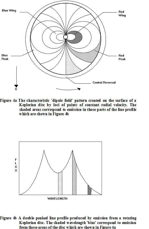
Figure 5 AX Per - 19/9/89

Figure 6 CH Cyg - 28/6/86

Maurizio started his talk by briefly discussing the connection between the Hubble constant and the age of the universe. The Hubble constant measured the expansion rate of the universe, and it was proportional to the inverse of the age of the universe. The precise numerical relationship between these two quantities (as well as the fate of our universe, that is, if the expansion would continue indefinitely or would stop and reverse at a given time in the future) depended on the density of the matter in the universe. This density could be obtained using estimates of the mass of clusters of galaxies.

The determination of the Hubble constant measured by the HST extragalactic distance scale key project, was based on the use of the cepheid Period-Luminosity relationship, established for cepheids in the Large Magellanic Cloud (LMC), and its zero point was determined assuming a LMC distance. However, this distance itself, was not yet precisely known. The value determined by the HST group was around 70 Km/Mpc/s, but the current uncertainty on the LMC distance caused an error of about 20% on this value.

An independent way to put limits on the value of the Hubble constant was through the determination of the ages of the oldest stars that populate our galaxy. These ages provided a firm lower limit to the age of the universe, and therefore an upper limit to the value of the Hubble constant.

The stars belonging to the halo of our galaxy were the oldest galactic objects. Many of them were contained in globular clusters,. Stars in a globular cluster all formed at the same time, with the same initial chemical composition (this could be determined from spectroscopic observations), and they were all at the same distance from us (since the dimensions of a cluster are negligible with respect to its distance). These properties allowed, in principle, a straightforward determination of their ages, by using stellar evolution calculations.

In order to determine the age of globular clusters, the Hertzsprung-Russel diagram of the stars in a given cluster had to be produced. This diagram was then compared to theoretical isochrones (the locus in the H-R diagram that was occupied by stellar models with the same age and initial chemical composition, and different masses). An example of this was shown in figure 1, for the metal poor cluster M6; the corresponding theoretical isochrones were shown. The position of the turn-off (the point which marked the end of the main sequence phase) was very sensitive to the age, and the comparison of the cluster turn-off absolute brightness with the theoretical one, provided the cluster age. One difficulty that still remained, was that the distance to the cluster was required, in order to get the turn-off absolute brightness. It looked like the problem of the distance scale could not be avoided.

In principle, one could use theoretical models of the horizontal branch (whose location was not affected by the a priori unknown age) to set the cluster distance, but there were still uncertainties involved, which caused an uncertainty of the order of about 2-3 billion years in the derived ages. Another possibility was to try to determine an empirical calibration of the RR Lyrae stars’ (which populated the horizontal branch of many globular clusters) brightness from local RR Lyrae with parallax distances, and use them as distance indicators.

Unfortunately, precise parallaxes for RR Lyrae stars still did not exist. Hipparcos had provided parallaxes for many thousands of stars, but the error bars on RR Lyrae stars were very high, so that there still were large uncertainties on their absolute brightnesses. The GAIA mission should provide much more accurate parallaxes, and solve this problem, but this not would not produce data for a least another 10 years or so.

A very promising way to eliminate these uncertainties, was to use well-detached eclipsing binary systems; these were two stars that were gravitationally bound, and which orbited around the centre of mass of the system, whose orbital plane was parallel (or almost parallel) to the line of sight. In this way, when one star passed in front of the other with respect to earth, we would observe an eclipse. The main idea was to derive the masses of the stars in the turn-off region of a globular cluster, provided some turn-off stars were in eclipsing binary systems. From the turn-off mass, the cluster age could be calculated using theoretical isochrones (see figure 2 for an example with the the M68 isochrones).

To determine the mass of the eclipsing binary components, it was necessary to obtain observations of both the light curve, and the radial velocity curve of the system, and Kepler’s laws could be used. Kepler's third law related the orbital period of the binary system, to the masses and separation of the components, so that if we knew the period from the light curve, then we would also need to know the radii of the orbits, in order to obtain the masses of the stars. This required both photometry and spectroscopy. When the spectrum of the system was obtained, absorption lines were observed on top of the continuum emission. If we fixed our attention on a particular line, we would find that this line was separated into two components, whose wavelengths changed periodically. The ‘movement’ of these two components (which produced the radial velocity curve) tracked the variation of the orbital velocity of the system’s stars, due to the Doppler effect. The analysis of the shape of the radial velocity curve, together with the study of the shape of the eclipses minima in the light curve allowed us to obtain, the shape, orientation, dimensions and inclination of the orbit, and the orbital velocities of the components. If, just to simplify the mathematics, we considered a system with circular orbits , using the first and third Kepler’s law together, with the information obtained from the radial velocity and light curves, we would get v1/v2=m1/m2 and (m1+m2)=[(4 pi^2)(r1+r2)^3]/(P^2 G), where v,m,r were the velocity, mass and orbital radius for the two components, P was the period of the system, G was the gravitational constant and pi=3.1415. From these two equations the masses of the components could be easily derived.

This method was recently applied to a system in the globular cluster Omega Centauri. However, due to the observational errors on the radial velocity curve, the masses were determined with a large error, corresponding to an error of about +/-3 Gyr on the cluster’s age.

In addition to the mass determination, the distance to the eclipsing binary could also be obtained from its light curve. In this case, by combining both the mass and distance information, the age of a cluster using both the turn off mass-age relationship and luminosity-age relationship could be obtained.

Moreover, if eclipsing binaries were observed and analysed in a large sample of clusters of different metallicities, then the absolute brightness of their RR Lyrae stars could be determined with precision when the clusters’ distances from the binary systems was known. This would provide a solid calibration for the distance indicator, that could then be applied , for example, to observations of RR Lyrae stars in the LMC.

The estimate of the system distance was obtained in three steps. The first step involved the determination of the radii of the components, which could be estimated from the duration of the eclipses (using the light curve), together with the known orbital velocities. When the radii were known, from the apparent luminosity of the components,the apparent surface brightness of the single components could be determined, that is, the energy emitted per unit time and unit surface.

The ratio between the apparent and intrinsic surface brightness of the components was proportional to their distance. The intrinsic surface brightness could be inferred fron their colours. In fact, for main sequence stars, empirical relationships (based on local stars with known parallaxes) existed, which linked a colour (V-I, or V-K, for example) with the intrinsic surface brightness in the V band.

If the eclipsing binary light curve was observed in different colour bands, the V-I (for example) of the individual components could be obtained, and then, using the local empirical relationships, their intrinsic surface brightness was derived. A comparison of the intrinsic and apparent surface brightness provided the distance.

Many eclipsing binary systems had been observed in other globular clusters (like 47 Tuc), in the galaxies M31, M33, the LMC and the SMC. They appeared to be probably the best tool to finally resolve the problem of the age and the value of the expansion rate of the universe.

Nick James asked what kind of accuracies were obtained when you used a big telescope to do these measurements? Maurizio replied that the masses could be constrained to about 1-2%, and that this translated to an uncertainty in age that should be around 1 billion years, assuming that the theoretical mass-luminosity relationship had no errors. The current uncertainties in age with the eclipsing binary method were around +/-3 billion years.

Richard Miles asked if reddening needed to be taken account of. Maurizio replied that it did need to be taken account of, but that Stromgren photometry could be performed to determine reddening, if it existed.

Norman Walker said that it must be difficult to pick out these stars in globular clusters as they the stars are very concentrated in these clusters. He also commented that the intrinsic surface brightness to colour relationship, that was used to derive eclipsing binaries distances was determined on local stars with a chemical composition that was different to the globular clusters one. Apparently, theoretical models suggest that the empirical relationships that are applied to globular clusters are negligibly dependent on the stellar chemical composition.

Maurizio replied that HST could observe globular clusters’ cores (and indeed discovered many eclipsing binaries in 47Tuc), whilst ground based telescopes had to concentrate on the less dense outskirts of the clusters. Even from ground based observations, eclipsing binary systems had been found.

Chris began by stating that he was hoping to cover the analysis of visual, CCD and photoelectric observations. He was going to spend most time on period-finding, as that was the sort of analysis that most people tried, and he would have a brief look at O-C diagrams.

He began by stressing that visual observations were very valuable. The eye was a wonderful detector; the only problem was that there was a brain behind it! All sorts of things affected the estimates that visual observers made - red stars, background light levels etc., which introduced complex biases into the observations. He illustrated the scatter that was typical of visual observations, by showing a light curve of T CrB, which spanned 1.5 magnitudes, rather than the few tenths of a magnitude that was its real variation. There seemed to be a personal bias for each observer, and this bias could be removed. He showed the lightcurve of T CrB folded with the orbital period, and this looked believable, but removing the personal bias of individual observers reduced the scatter considerably. Cleaning up the observations in this way makes detecting periodic variations more reliable.

In general, photoelectric photometrists used filters, so that their results were more or less consistent with one another, but CCD observers quite often didn't use filters as they wished to maximize signal levels. Chris showed some data for one of Bernard’s variables, BrhV65, as derived by three different instruments. There were several ways of aligning the data, but it was impossible to tell which gave the ‘right’ light curve. So it was not possible to combine these data to tell, unambiguously, what type of star the light curve indicated. Chris made a plea for people to use filters for this type of work whenever possible. He added that whilst it was not always necessary, if you were intending to combine your observations of a low magnitude variation star with the measurements of others, then it helped a lot to have used a V or R filter. You didn't lose as much light as you thought, and it was much easier to combine the data.

Period finding had always been regarded as something of a black art. This involved taking data, folding it with a number of periods, and using a period-finding technique to construct some measure of the goodness of the light curve. In most cases the measure could also be interpreted as a probability that the period found was not just due to noise. Many methods had been used, but the most popular included Phase Dispersion Minimisation (PDM), Discrete Fourier Transform (DFT) and Least Squares methods, in various forms. Autocorrelation was a related technique that could provide additional information.

In the PDM methods, the folded light curve was divided into a number of bins, and at the best period the dispersion in any particular phase bin should be the lowest. There were several different methods of calculating this statistic. The advantage of PDM methods was that they worked on any shape of light curve. Software for PDM methods was also freely available; PDMwin3 could be obtained from VSNET, and a DOS version was also available. PDMwin3 used Stellingwerf‘s method, which produced the 'theta statistic', a measure of how reliable the period you had found was. A problem with PDM was that there were several different methods currently in use, which produced different statistics, so that you needed to be careful when comparing results with others. The periodogram was not unique in that the bin structure and the number of covers (bin offsets) you had chosen to use, affected the final answer. Although PDM software was freely available, it frequently crashed Chris's computer!

The Discrete Fourier Transform method worked in a different way: for every trial frequency, it tried to determine the amplitude of the fourier component at that frequency. Something that was a pure sine wave would have no power except at the period that was present. This method tried to determine the power at each frequency, on the assumption that it was looking for a sinusoidal waveform. This method was quick and easy to program. The minus points were that DFT was sensitive to sinusoidal variation; it was based on a mathematical approximation that assumed that the data were evenly spaced, which was not usually the case, and you could therefore get spurious answers. There was also a problem with aliasing.

The Least Squares sine periodogram method was an honest method. It folded the data with a certain period, fitted a sine curve, and told you the residuals from this fit. Where the residuals were minimised, was deemed to be the best period. One of the main disadvantages to the Least Squares method was that it was slow, and sensitive to sinusoidal variation, and had the same aliasing problems as DFT.

There were other methods. Wavelet analysis was a bit like DFT, but could focus on a range of time scales, and provide much more information about the phase and amplitude variations of the periods in the data. It was a very powerful technique, but there were a lot of parameters to set up, and a lot of starting points to choose from, so this technique was not for the faint-hearted! The Lomb-Scargle method was a cross between DFT and LS and gave an answer equivalent to LS; this was not widely used, as there were not many programs easily available; Clean was developed from a 2D method that was used for cleaning up radio maps. There were also programs available that were based on neural networks (see VSNET website for the Lancelot program); neural networks were very powerful, but you needed to understand what you were doing.

There were some common difficulties with analysis, that the users of these programs must be aware of. Aliasing was an effect that produced spurious features in the periodogram, and was purely due to the data spacing of the observations. If you had a sine wave and the data was taken at one-day intervals, the period-finding method would fold the data with that period and get a good fit. If you fitted another cycle into this, you could also fit the data, so that a period of one cycle per day different would also come out of the analysis, which was the frequency of taking the observations. The data could also be equally well fitted by a period that was 2, 3 or 4 etc cycles per day different to the real period, so you could end up with a series of spikes to higher freqencies, and it would be difficult to tell which was the true period. The aliases also ran towards lower frequencies but were apparently folded back at zero frequency, to produce a second series of spikes running through the periodogram.

The nyquist frequency was half the dominant data frequency, but strictly only had a meaning when in regularly spaced data. The effect of the nyquist frequency was that you had no information on frequencies higher than the nyquist frequency, so in practice the periodogram was apparently reflected about that point. If you wanted to avoid aliasing, you needed to observe randomly, and this could be achieved by observing at larger hour angles.

Chris added that there was a periodogram of the data spacing called the window function, which told you what aliases you were likely to see in your data due to data spacing, and this was easily calculable from the DFT programs.

Chris moved on to examine some real data using photoelectric photometry of XY Lyr, which had errors of the order of a few hundredths of a magnitude. There was clear variation of this red star, with a period of around twice the range of the data. Using the least-squares periodogram it was possible to see this period, but there was also another period at around 120 days. It was possible to remove these periods and look at the data again. The longest period was very difficult to remove, as there was only half a cycle present in the data but in the end it was possible to remove five periods and still be left with others that were well above the noise. It was impossible to tell whether these were real, or whether they were noise. A five-period fit did a reasonable job of fitting the light curve but was not perfect. With this type of star, you knew that there was a possibility that the periods and phases were changing. You could fit a static solution, but this told you nothing about whether the periods were changing or not. This was a case in which wavelet analysis would be useful. For long period variables you could quite often get a cluster of spikes around a particular periods, which was a good indication that the period was changing.

Chris moved on to describe the autocorrelation technique in which the data (evenly spaced) was taken, stepped across and 'slid and compared' to see how well the shifted set correlated with the unshifted set. There was a close relationship between this and the other techniques, as the periodogram was the FT of the autocorrelation function. He demonstrated this method with mu Cephei data to show the persistence of the periods

O-C diagrams were useful for looking at period changes. Miras, in particular, had period changes that could be very large, and these could be seen directly in the periods themselves. O-C diagrams could follow smaller and more complicated period changes. It was often possible to see very small period changes as they accumulate in O-C diagrams. Cepheids and other pulsation variables, and eclipsing binaries showed changes due to changes of internal structure or dynamical changes that could provide important information. In these diagrams you looked at the difference between the times of maximum or minimum light that you saw, and what was expected on the basis of a constant period. Period changes appeared as a characteristic parabolic line in the O-C diagram and you could calculate the rate of period change through the curvature of the line.

Chris closed his talk, by reiterating that visual observations were a very valuable resource, and could be corrected to improve the data by removing personal bias. He felt that if observers wished to perform photoelectric or CCD photometry then the use of a filter was very important to data analysis. He felt that it was important to have data analysis and observations feeding each other. If a quick analysis was performed early on in the observing history of a star, then it was possible to predict when observations would need to be made, and this might enable results to be obtained much more quickly.

John had used the AMPSCAN program for analysis for many years. For working out periods, this used a discrete Fourier analysis approach, which took the magnitudes and sometimes binned them; this involved taking 10 or 20 nights' observations, perhaps, and averaging them up. The binning process sometimes reduced the aliasing that you could get by having too much data in one or two places. If you did have too much data, it could be better to select one representative point per bin.

It was also useful to plot the amplitude and phase on a polar phase plot. In some cases the amplitude and phase were changing in some way, and the effects of aliasing due to this might be removed in this way. Sinusoidal changes in frequency could also be removed using Bessel functions.

John went on to examine some UU Aur data; this had many gaps and it was difficult to tell by eye, from 30 years worth of observations, if there was any pattern to the data. John said that he had put the data into bins so he had 10 day means; the gaps were still there, but they were less conspicuous, and some kind of periodicity was already evident. A semi-amplitude spectrum analysis for UU Aur using this data, showed periods that agreed with the AAVSO analysis.

John said that he had been working with Kevin West on RR Umi. John showed the analysis of his own data, from which he deduced a period of about 33.56 days, which was only just above the noise. He then received Kevin's data (see VSS Circular, 101, p8), which looked a good deal more promising, and tried analysing this, and he got a good period of the same value (33.56 days). There were six years between the end of John's observations and the beginning of Kevin's. John then obtained all the BAA results (digitised thanks to the efforts of Terry Miles), and these showed the same period, although now a few other periods appeared, presumably because with more observers, there was more noise present. John said that he hoped that it would be possible to produce a paper together with Kevin West showing the analysis of this data.

In summary, it seemed that AMPSCAN gave consistent and accurate results. John wanted to stress that visual observations were still very valuable and worthwhile, particularly when done regularly over a long span of time, and that observers should continue to contribute their observations to the database.

John proposed that four areas be covered during the discussion; these were international standardisation of sequences, CCD charts, sequence selection and coloured comparison stars.

International Standardisation of Sequences.

The BAAVSS was formed in 1890, and had adopted the best procedures and sequence information that was available at that time. The same procedures were valid today in most instances, but there were problems with the sequences. The problems stemed from the fact that amateur variable star observers around the world today were fragmented into around half a dozen groups, that had developed their own individual sequences. This meant that several sequences could exist for the same stars being observed and this caused problems when analyzing data derived from the different groups. Recognising this as a worldwide problem, the BAAVSS and AAVSO had begun a dialogue with a view to standardising sequences internationally. This dialogue had accelerated within the past 18 months with a series of meetings. The intention was not to use the same charts and to agree to adopt the same procedures universally, but to ensure that the sequences which were used did not differ significantly for the same variable star. It was considered best to concentrate on obtaining agreement amongst the Anglo-Saxon groups first (AAVSO, BAAVSS, RASNZ, TA), as agreement amongst them was thought to be the most easily achieved and their databases constituted approximately 80% of the amateur variable star observations made within the last 100 years. Each of these groups had exchanged copies of their charts, and had agreed to circulate to each other, any future charts that were drawn up. Since there was little duplication between the BAAVSS, RASNZ and TA charts, we needed to concentrate on comparing them with the AAVSO charts and this was being performed as follows:

AAVSO / BAAVSS charts Checked by BAAVSS (J Toone)

AAVSO / TA charts Checked by TA (G M Hurst)

AAVSO / RASNZ charts Checked by AAVSO (M Simonsen)

Of the 1,000 AAVSO charts and 400 BAAVSS charts that had been compared, only 141 had been found to be covering common variable stars. Of these, 59 were found to have significant differences that required investigation (significant differences meant 0.2 magnitudes or more). These were currently being investigated, and a report with recommendations for eliminating these significant differences would be presented to the BAAVSS and AAVSO shortly for their consideration and hopefully rapid implementation.

At this point, Keith Robinson asked if roughly the same sequences were being used. John replied that the AAVSO had, in the past, tended to measure many of the stars around a variable for use, whereas the BAA measured and used just a few. The standardisation process involved comparing only those stars that were commonly used.

Nick James asked how many charts had changed so far as a result of this. John said that he had changed around 6 BAAVSS charts so far, in advance of the report being issued.. He was starting to use Tycho 2 (Vj) magnitudes down to magnitude 11, and after that he would use CCD V measurements. This had been agreed with the AAVSO as a future policy, to ensure that when new charts were produced, the sequences should not differ between the groups. Chart formats would remain as they currently were, as they worked well with the individual groups’ procedures.

Norman Walker suggested that an image of each star field with BVRI filters should be obtained to get accurate magnitudes. John mentioned that this was what Arne Henden was already doing. Norman suggested changing the system to do this, rather than using Tycho 2 (as Tycho 2 magnitudes are only accurate to a few tenths of a magnitude), so that you would have a good measurement of magnitude on a standard (Kron-Cousins) system.

Keith Robinson asked if, after all these sequence alterations were made, the light curves would have to be redrawn. John said that as the BAAVSS recorded the full estimate for each observation, we could easily change our light curves. Keith was concerned that professionals would receive data from different groups, and would need to do a lot of fiddling around to make them consistent. Nick James asked if the AAVSO perhaps didn't want to change their system, as they didn't record the full estimate. Gary Poyner felt that it was important to move forward quickly, and said that he felt that this was all moving very slowly, but John said that this was now progressing well in spite of recent computer problems. It was suggested, by an audience member that we might consider including individuals colour bias as well, but Hazel McGee suggested that it would be preferable to supply this information to professionals who required the data.

John said that as the AAVSO had formed early (1911), and were the biggest organization, most other groups that had formed later, had adopted the AAVSO as a role model, and had followed their methods and formats. Nick James felt that the AAVSO had no reason to change, as the professionals preferred to take data from them as they had more data points. It was also noted that the AAVSO would have difficulty in changing their sequences, because of the way their system worked. It was felt that the best option for the AAVSO would be to change the way they do things and record the full estimate. Norman Walker mentioned that the AAVSO took out observers’ personal biases. This information was then used for period change analysis, and he felt that the accuracy was not there. Norman still felt that we should do this right and use a CCD-obtained sequence. John Saxton felt that we should record accurately what had been done, and which sequence we used, and then we could sort out the sequence problems in our own time.

John asked if it was considered necessary to produce charts for CCD observers, and if so, how should they be produced? Denis Buczynski felt that for new eruptives, a graphical representation was useful, but that for stars that were being monitored regularly over a long period of time, it wasn't necessary. Nick James thought that a chart was not necessary, just some photometry in V and R for a number of stars, so that the calibration of the camera and linearity could be checked. It was possible to download GSC or DSS images/Vizier, to find the star, so that a chart was not required. John suggested that we should try to provide information on the web page in tabular form. This would include the identifier (GSC) of the comparison star; whether it cross-referenced to a lettered sequence chart; the position of the comparison star; the comparison star magnitude to 2 decimal places (but Norman thought that 3 decimal places was necessary); and the magnitude error for that measurement. Also the B-V value for the comparison should be included. Nick James thought that you would need BVRI magnitudes for each star. Richard Miles mentioned that you had to be very careful to pick comparison stars that were not contaminated by faint field stars in the background. He said that a deep sky image like Palomar needed to be used to ensure that there was no contamination. But at the same time, there would need to be enough stars to accommodate both small and large field of view systems. Nick James thought that stars would be required every two magnitudes. Richard thought that CCD observers should report both the magnitudes and the error bars as well. Nick James and John were in agreement, that the BAAVSS needed to be in touch with the AAVSO on this issue, so that we were not duplicating our efforts and developing separate CCD sequences. Guy Hurst expressed concern that there seemed to be a lot of variation in the V measurements that were currently being reported. It was stressed that the instrumental calibration needs to be done in order for all measurements to agree.

The point of major concern regarding sequence issues was that of the selection of comparison stars to be used in the future. This had been discussed with the AAVSO. Future charts would use Tycho2 (Vj) for stars down to magnitude 11 and CCD V measures for fainter stars.

The issue of the use of microvariables was discussed. John said that we could retain microvariables (<0.1 magnitude range) as comparison stars on visual sequences, provided that they were not orange or red stars. In exceptional cases we could accept a 0.2 magnitude range if there were no suitable alternatives (CH Cyg comparison J for example) or if the change would introduce more potential errors. The scatter in visual data was currently as high as 0.5 magnitudes (particularly for red stars), and the use of such microvariables might increase the scatter further. John stressed that in the ideal case this wouldn't be done, but it might be necessary on the odd occasion, and that this would introduce a systematic error. Nick James pointed out that the microvariable changes might be picked out during data analysis.

Some previous BAAVSS charts had listed magnitudes to 2 decimal places, and in future it was intended that 1 decimal place should be used, and that sequences would be constructed with about half magnitude gaps between the comparison stars.

Another question was that of whether the Howarth and Bailey formula; mv = V+0.16(B-V) should continue to be applied to convert V to mv. Roger Pickard preferred that it only be used for data analysis and not on sequences. In the past, many of our sequences for dwarf novae had already applied this formula, and although some of the sequences were considered poor, others seemed better than the equivalent AAVSO sequences. John pointed out that it would be necessary to revisit many sequences if this formula was removed. It was agreed that the sequences for which this formula had been applied, should be revisited. However, if a V to mv formula was to be applied for the purposes of international standardization of sequences, should the Howarth and Bailey formula be used, or that adopted by the AAVSO [m = V+0.182(B-V)-0.15]? John felt that most of the sequences that we had applied the Howarth and Bailey formula to, looked pretty good with a few exceptions. John said that further work was necessary on this, as it was fundamental to the sequence standardisation process.

Other important criteria for the selection of comparison stars was to avoid stars with close companions and to always check their colour.

The AAVSO still advocate that comparison stars should ideally match the colour of the variable providing the B-V did not exceed +1.5. John expressed mild concern with this, when dealing with red variables. John stated that most sequence queries that were received from observers, centred around comparison stars of differing colours, usually involving blue and orange stars. The best way to mitigate the risk of problems was to limit the colour range of comparison stars wherever it was practical. John proposed limiting the B-V range to 0 – 1, with extremes of 0 – 1.5. Stars with a B-V of greater than +1.5 had a very high risk of being variable themselves, and in some cases the variability could be intermittent. Stars with a negative B-V should also be avoided because they were particularly susceptible to extinction effects. Guy Hurst felt that we should push the AAVSO to follow us on this issue. Guy didn't like the way the AAVSO picked red stars to compare with novae on decline; he believed that very bad light curves were obtained as a result of this.

Chris Jones expressed his concern that there was a huge backlog of charts to be looked at, and asked if there would be a delay in the issue of new charts due to lack of time, and the need for CCD measures of magnitude 11 and fainter stars. John suggested that if people were willing to help produce charts in the right format, then this would assist, and Henden and Skiff were coming up with many CCD sequences that we could use. Chris thought that Henden was keen to produce sequence information for CVs, but was unlikely to produce information for Mike Collin's stars. Guy mentioned that he thought that the recent AAVSO charts (produced from the A2 catalogue) had some very peculiar star details, and John agreed to look into this.

There followed a fascinating trip to the observatories. There were a number of domes, but I know no one who went on the visit, who failed to be stunned by the sight of the 'multiple mirror telescope' which consisted of 7x 16" schmidt cassegrain telescopes, all on the same equatorial mount! This is currently unfinished, but it is hoped that they might see first light some time this winter, and then the mirrors will be sent away for re-aluminising before the telescope begins its work proper. The plan is that fibre optic cables will take the light from the telescopes to a spectrometer. It is to be used by Gordon Bromage to back up XMM observations of flare stars, and for final year undergraduate use.

After yet another excellent meal the BAA president, Nick Hewitt introduced our speaker of the evening: Dr Alan Chapman speaking about 'When amateurs ruled astronomy’.

Alan began by asking the question 'Why did we have the golden age of astronomy in the nineteenth century?' At that time, people might have occupations in astronomy but they did not have jobs. They could be defined as 'the grand amateurs'. Part of the answer, to this question, was that money and pensions meant far less at that time. Science was financed in a very different way to the way that it is financed today. In those days, you only paid for the things that were entirely necessary; work that was intellectually valuable, but not essential, would never be financed. The only jobs that were paid jobs, were those jobs that were paid for by the state.

In 1660, the Royal Society was founded; it was the first professional society in Europe. However, the society had no funds, and needed to collect a shilling a week to pay the bills. Other societies followed in a similar vein, being founded with royal charters and status, but not a penny to their name. It seems clear that at this time there was no tradition of having centrally funded science.

In other countries abroad, however, this was not the case. There were places, such as the St Petersburg or Berlin Observatory, in which, if you were reasonably well educated, you could aim for a job as a director, with a pension to follow later. In these countries the money was raised to fund these observatories by taxing the poor. So why was it that this did not happen in England?

Charles II was wise enough when he founded the Royal Society, not to tax the poor, but to ensure that the Royal Society understood that they must raise their own money to pay for any research. Later on through the eighteenth century, there was the energy and the cash to develop the industrial revolution, but the money stayed in people's pockets; so if you had an idea you could develop it. In this way, a deeply capitalist economy emerged. The English people had the freedom to do as they wished, and foreign visitors noticed and commented on this. In England there was a different attitude to talent, than that found abroad. You didn't take money out of the economy, but left it there to do what it liked. As England also had the biggest middle class in the world, many people just lived off their dividends. This created a pool of people with a good education, and this was the beginning of the age of 'grand astronomers', some of whom Dr Chapman went on to describe.

Sir James South started in the medical profession; doctors in this age could earn a great deal. By 1816, South married the daughter of a brewer (brewers also earnt a great deal of money at this time and his wife brought an income with her of £8000 per year - equivalent to perhaps £200,000 today). Frances Bally was a London stockbroker who founded the RAS; in fact, the first address of the RAS was the London Stock Exchange. Another well-earning occupation was that of lawyer. Lee was a lawyer who built one of the finest observatories in England. Naysmth retired at the age of 48, taking over a quarter of a million in cash from his business (he owned a foundry in Manchester). Another potentially well-earning profession was that offered in the church, which had about ten to twenty thousand clergy at that time. There was no standard pay structure, but a handsome income, and moderate work could often be had. Furthermore, it was possible to rise to a career in the church from lowly beginnings. The Reverend Pearson came originally from Cumberland, and was educated at grammar school, the son of a farmer. He later went to Cambridge and discovered that he had an ability as a public lecturer in natural philosopy and astronomy. He started to make up to £1000 per year from talks. He also picked up two clerical beneficiaries from his college, and had many letters after his name by the time he retired. This was a society that encouraged brilliance; your background was irrelevant.

Greenwich was a rare institution, in that it received funding for the task of working out how to find the longitude at sea. Flamsteed, Halley and others had all failed. The John Harrison finally succeeded because he had the instruments necessary to do the job, and in 1749 he received the Copley medal of the Royal Society, which was the Nobel Prize of that time. In 1764 William, his son, was also elected as a Fellow of the Royal Society. These men moved in this open elite without barriers.

People at this time used the word 'amateur' proudly - in the Latin sense of the word - to love - to be an amateur astronomer means that you love astronomy. At this time paid astronomers didn't have status; they were considered equivalent in status to a groom or a lawyer's clerk. The people who had the esteem, the likes of the Fellows of the Royal Society, were the amateurs. It was assumed that by the time you were able to join the society (requiring that you were able to pay your 40 guineas subscription, and have sufficient friends who were already members to be able to nominate you for membership), you had the education to know what was worth researching.

There was a body of men who knew what needed to be done. They published in the major journals, and they travelled to collaborate with other astronomers abroad. Many astronomers knew each other very well; so well that when Struve had been staying with Lassell and left a shirt behind, Lassell sent it by 'Airy' post some days later, when Airy was travelling from Lassell's house up to London. Cooperation between astronomers had to be voluntary, but where it existed, a good railway system and cheap post meant that you could correspond almost as quickly as you can today.

Dr John Lee lived at Hartwell house, which became a centre of English Grand Amateur astronomy. Anyone who was anyone, turned up at Hartwell house and signed the ledgers on arrival and departure; much information can be gleaned from these ledgers today. Baden Powell mentioned in such a ledger, that when the sun was shining in, he used the mirrors at the end of the room and a prism to see 'Fraunhofer's lines'. The Hartwell House observatory was about 10 feet from the house, and was connected to it by a passage from the library. Apparently Lee was observing Venus one morning in 1845 with the 6" refractor, and noticed some spots on Venus. He thought that they should let Airy, the Astronomer Royal know, so the next morning they chartered a train to go to London to tell him!

The grand amateur league also hosted some battles. What these gentlemen regarded as important were gold medals and honarary degrees; they loved letters after their names. This meant more to them than their jobs did. They often fought and disagreed with each other. South famously fell out with Airy and Troughton (who manufactured astronomical instruments). South paid £1800 to Troughton to make him an equatorial mount for a large telescope. Troughton didn't want to build it to South's design, because of a number of design faults that he could see. However, South convinced him to go ahead, and build the mount according to his specifications. When it was built it had all the defects that Troughton had said that it would have, and South refused to pay. Troughton sued. The whole of the RAS took sides in this argument. Eventually after about six years going through the courts, it was decided that South must pay. In a fit of rage South smashed the mount up, and then issued a handbill to the scrap merchants that they could take the scrap metal. It seemed, at this time that South was almost going mad; had he not been a knight, and had many friends, he would most probably have been certified mad. During this time he started to write letters to The Times newspaper, airing many bad feelings.

Binary stars were a passion at this time, as was the question of the size of the universe, and whether the nebulae in space were part of a big cluster. Some people thought that with a big telescope you might be able to break down the cluster of stars into smallers ones, which would suggest that the stars were not all that remote. It was at this time, in 1845, that Lord Rosse built his telescope, whilst acknowledging that he would get few hours use out of it due to poor weather. Planetary nebulae also fascinated these astronomers. Why did you have a glowing circle with a star in the middle? Variable stars were a great subject of interest, together with the dynamics of the solar system, and how many satellites were going around these other worlds. At this time, you couldn't explain things so well, but you could collect the data. The revival in the study of sunspots was made around this time, and Herschel became concerned with how the sun burned, having seen deep chasms in the sun's surface. Naysmth suggested that perhaps a kind of volcanic vortex came up producing a willow leaf granulation. They imagined, by this time that the sun had an atmosphere pitted with sunspots, and a blast furnace below. Naysmth who owned a blast furnace, even tried experimenting with hot gases and metals in the furnace.

The spectroscope was first used by Bunsen, in 1859. Two men, Huggins and Lockyer first developed the use of the spectroscope. Huggins suddenly discovered gas in nebulae, and he was the first person to show that the stars have different chemical compositions, and that star clusters and nebulae are different. Lockyer, a wealthy civil servant in the War Office, bought a Cooke refractor; then, having read of Bunsen's work with the spectroscope, he obtained one, and did the first spectroscopic work on sunspots. He was elected FRS whilst still working at the War Office.

The professional astronomers were only awarded money to do work once the amateurs had already blazed the trail. Astronomy was a passion to many victorian astronomers such as John Jones who worked at a slate counter at Bangor Docks; he made a 8.25 inch reflector and a spectroscope although he earned very little. In the early 1930s, George Orwell wrote 'Down and Out in London and Paris'. Whilst In London he did a stint as a tramp. He mentioned a man whom he encountered in a doss house, whose nickname was Bozo. Bozo had done painting in Paris, he limped badly, probably had consumption, and worked as a pavement artist. He often painted pictures of astronomical bodies that he had seen in books. He said that he had often seen Jupiter, Saturn and Mars, and he wondered if there were people on those planets freezing as he was. He condemned his fellow tramps for being brain dead, and felt he should fight to maintain his interest in these things.

Dr Chapman finally showed some slides including several of Dr Lee, and Hartwell house. One of the slides showed Dr Lee at the telescope wearing his observing hat with tassels and signs of the zodiac decorating the hat.

There was also a slide of Lassells giant telescope which was the world's first big equatorial reflector. Lassell shipped this to Malta together with his family and grand piano for five years. He felt that people in Malta considered him to be an eccentric amateur, going over there, as he had, purely to observe the skies.

There was a slide of the first telescope that was ever built for the first serious use of astrophotography by Warren de la Rue. There was also the steel manufacturer, Henry Bessimer, who was a multimillionaire. He lived in London and had a vast estate, on which he built a forty foot focal length ‘Nasymth’ telescope. The whole observatory rotated so that he could view from one place.

Nick James thought that the story of South was amazing and Dr Chapman confirmed that if South hadn't had so many friends then he probably would have been certified mad. South spent a lot of time with the Earl and Countess of Rosse who treated him affectionately, rather like a respected, if difficult, elderly relative.

Gary said that he had been intending to cover observing problems, but that as many of these things had been covered in the chart session yesterday, he had decided to cover data entry instead. He explained that he sent data to multiple organisations by entering his data into one line of Excel, and exporting it in different formats for each organisation. Data only needed to be entered into one or two fields in the main sheet, which drew data from a look-up table to complete the remaining entries automatically. He said that he entered the data into the star column, and the spreadsheet entered the designation automatically; he entered the date, and it entered the JD; he entered the time, and the decimal UT was worked out. It also entered the sequence details for the star in question. The spreadsheet automatically entered all of this data into the TA and AAVSO sheets etc. Gary said that he had offered the AAVSO all the data, but that they only wanted the magnitude and star name, and did not require sequence or any other information. The AAVSO now accepted data from Gary directly from his spreadsheet, but only the magnitude and star name. Hazel McGee said that since last year when the submission process had been changed, the chart information was now also submitted with magnitudes, and that the AAVSO now provided a program that would convert VSNET formats to AAVSO formats.

Gary felt that it was important not to have to enter data in several different formats after an observing session, and that this system therefore worked well for him. In Gary's opinion the BAA format did not work well now, and the BAAVSS should consider accepting single line entries. In this case it would be possible to give people Excel templates to use. Gary added, that in receiving observations for TA, he received about 10 different formats. He was thinking of insisting on a single line format entry, and offering a four month changeover period, after which observations would only be accepted in the required format. Guy Hurst thought that instrument information, and the times of observation should be included in the report, but Gary felt that this could go on the end. Norman Walker suggested that a common format for both visual and CCD observations was desirable. Hazel suggested that we should be given a format that we should all just stick to. With the BAA current system we had a header and the observations under that header, then another header and a series of lines. Roger agreed that when he was passing on the SU UMa observations to Darren Baskill, he had had five different observers sending in data in five different formats. Nick James remarked that if we had a one line format then it would be easy to write a script to generate that format from any other one line format. Hazel said that she had managed to get Excel to reduce the magnitude for her, by just doing the arithmetic. Phil Busby suggested that when we had decided on the template that it should be on the web site for downloading, but Gary said that it was already on his own webpage. Chris Jones had written a similar thing for Lotus 123 - and said that it was on the AAVSO web site. Hazel suggested that instead of fiddling around with paper and pen and torch to note observations, a small digital recorder was more useful, and particularly for meteor observations. Gary thought that the digital recorders were also very useful for eclipse observations.

Melvyn began by suggesting that the binocular programme probably needed a bit of revision. The programme originated in the late 1960s, was modified in the early 1970s, and it was hoped at that time that the binocular programme would help to increase the popularity of variable star observing. The programme had many red stars: AH Dra had an amazing light curve; XY Lyr was very underobserved; RR UMa was taken on, as it is so bright, but the scatter turned out to be huge. John Howarth had showed that with analysis of Kevin West’s photoelectric photometry, you could do a lot with the data.

In the recording of observations, bias was a very important area. Bias could not be taken out of the individual equation, and we all needed to look at our own observing, and do what we could to minimise bias.

In considering the practicalities of mounting binoculars, Melvyn showed a picture of a chair with a binocular holder, plus a tripod with binoculars mounted on top. Roger commented that he found holding binoculars difficult, and felt that they need to be mounted in this way. Denis asked about the Canon image stabilised binoculars, and wondered how good they were. Melvyn had found that there was a significant magnitude advantage to be obtained when viewing with stablised binoculars, and several others in the audience agreed with this. Guy also asked if people were advised to put their backs against a wall when observing using binoculars, as this improved the accuracy of the estimate; Guy felt that he gained a magnitude in this way. Melvyn did say that hand held binocular observations did produce more scatter than observations made with a fixed instrument. Gary commented that the finderscope on the telescope should not be underestimated, as it was often as good as a pair of binoculars. Keith Robinson wondered if there was any known effect on accuracy, of using one eye rather than two. Melvyn did not know the answer to this, but felt that it was a question that someone must have examined.

It was noted that there were a number of very under-observed stars on the list. The Z And type star NQ Gem was an important star that only had a few observations in the database. Being very close to three 7^th and 8^th magnitude stars in Gemini, its observability was difficult and coverage was minimal. It was felt that these very under-observed stars should be noted in the next circular. Melvyn said that some of the lpvs/miras were also under-observed. Chris wondered if the 'under-observed' list that used to be published some time ago should be reproduced again.

Melvyn suggested that there should be a re-examination of how interested professionals were in the data, and to see if there were other stars that they would be more interested in, that were not currently being examined. Chris Lloyd thought that some of the low amplitude stars might be a bit suspect, and that stars that were both low amplitude and irregular probably weren't going to benefit much from being observed. Any stars that had shown intermittent changes, however, should continue to be followed. Chris added that observers should make sure that they observed as consistently as possible, and should not try to guess their own bias, as this was not possible. Roger added that before the binocular programme was updated, some analysis needed to be done so that we could see what needed to be dropped.

Norman felt that when you had a lot of data with a periodicity, you could get down to a few hundreths of a magnitude if you had a lot of data. Gary noted that the observation and analysis of observations made of the same star, with both binoculars and a telescope was a problem and should be avoided at all costs. John Toone asked if it would not be worthwhile putting a note in the circulars when an SRb entered an active phase, so that people might be encouraged to observe these stars; he felt that these were especially good targets for new observers. Norman said that he thought that it was still important to monitor stars, even when they appeared not to be doing anything, as the quieter phases could often contain information. Hazel pointed out that when a star was doing something, it was more interesting, especially to new observers. Chris felt that resilience in observing needed to be reinforced amongst new observers. Hazel said that the BAA were going to start issuing e-circulars and this sort of thing could be reported through them.

John asked if there was any news on the binocular observing book coming out, that the VSS had planned for some time. Roger noted that all the leaflets had been combined and edited, and that it had come back from the printers. The book included an introduction to the section, a chart catalogue, about two dozen charts and some light curves.

Norman wanted to point out that Kevin West's work was outstanding and should be encouraged. Norman had received some of Kevin's data some to analyse, but hadn't had time to look at it properly. Chris LLoyd agreed that Kevin's work was all very good.

John Saxton gave a quick update on the position of the computer database. He said that he had done most of the hard work, and could now read the standard VSS reporting format, but that if it was decided that a different reporting format would be adopted, he would be happy with this. Hazel felt that John should just specify his preferred format, and observers should stick to it; Gary agreed that once decided, it should be made official and included in the new observing guide. It was agreed that the CCD reporting format would be decided upon at a later date. In answer to Gary's question regarding uploading of light curves to the web page, John thought that he would be able to generate the light curves, and e-mail the data to the web pages once a month.

Tom Lloyd Evans was struck by AF Cyg light curve that Melvyn showed; he wanted to stress that professionals were only recently starting to become intersted in these stars. He mentioned that five period luminosity relations had been found when looking at the LMC, but that it was very important to get good observations of stars in our own galaxy ,as these were the ones that could be studied in detail.

Electronic Observing by Nick James

Nick wanted to show some of the techniques that he used for producing magnitudes from CCD images, but he first addressed the question of why filters should be used, by showing several graphs of QE (Quantum Efficiency) vs wavelength for different CCD chips, which illustrated the vast variation present in response, between different types of chip. He explained that, if unfiltered photometry was perfomed, different results would be obtained from different cameras for different coloured stars. Filters either needed to be carefully matched to the CCD response, or careful calibration should be conducted.

Nick then showed a frame of WZ Sge, which had an annoying star very close by. He explained that thermal noise affected CCD images, which took the form of a dark current. If a dark frame was taken (a frame with no image), then this could be subtracted from the raw image to subtract the dark current. As dark current scaled with temperature, it was important to try to keep the camera at a constant temperature, but if the temperature did vary, then software was available that would scale the dark current according to temperature.

Nick demonstrated the importance of calibration using a flat field, by showing a 'flat field from hell', which was an image that was taken through a dirty filter. The flat field was important as the CCD was not equally sensitive across all pixels, and optical effects also affected the image. There would obviously be a significant variation in sensitivity, if one of the imaged stars was in the middle of a 'donut' and the comparison was not. The stars might also be drift across different areas of sensitivity. The flat field would be taken in twilight, or by using translucent illuminated screens across the telescope. Nick stressed that it was very important to take dark frames and flat fields. Roger also mentioned that you needed a flat field for each filter, unless the filter wheel could be accurately positioned each time. Chris Lloyd noted that it was very important to use a multi-chromatic light source for the flat field.

For processing his images, Nick used Christian Buil’s software - IRIS. In order to do a reduction of a CCD frame, you had the benefit of being able to chose from a huge number of comparison stars. Nick's software took the best fit through all of the available comparison stars. The computer automatically compared the stars that Henden had measured, to those that Nick had in his field. In this way it was possible to use a lot of stars, and any stars that appeared odd in behaviour, were immediately apparent, and could be excluded as comparisons.

Nick outlined the two main types of photometry that were commonly used. In 'aperture' photometry, an aperture was set up around the star, which allowed the measurement of light from the star in the central region, and light from the sky in an annulus around the star. This was a good method, but proved difficult to use for WZ Sge, due to field star contamination. An alternative method was 'point spread function photometry' (PSF), in which images were processed to obtain a 3D gaussian profile of the light intensity. Nick explained, that in his case, the stars were fuzzy, and the PSF was far from ideal, as he was oversampling the star image, and had telescope drive inaccuracies associated with his system. Once the PSF had been determined, then the software fitted this PSF to the stars to be measured, which enabled an accurate determination of where the star's light ended to be calculated. This method worked particularly well in crowded fields.

Nick had made an evaluation of his unfiltered performance of his CCD camera, (an R-401E camera based on the Kodak KAF-0401E chip). In the WZ Sge field, he took images that were unfiltered, and over a five magnitude range he got the computer to identify stars that were common to both his image and to Henden's list. He then plotted the difference between his derived magnitudes, and Henden's magnitudes, and found that there was a difference of about -0.1 magnitude in the V band, and about +0.2 magnitude for the R band stars.

If photometry of CVs was performed, it was relatively easy to end up with a considerable amount of data. Nick said that when he first started to do this type of work, the programs that were available to batch process data were limited. Nick's software took a list of objects in the last frame, and a program was used to obtain the coordinates of the objects. A file was generated which contained a list of the apertures that you wanted to use, then when the program was run, it would step through all of the frames, reducing them each in turn. This worked well, unless there were large shifts between two frames. The software provided numbers of counts for each object, and a time. You could then import this into Excel to process the raw counts in order to obtain magnitudes. The batch processing program could also remove dark frames, and divide flat fields.

Peter Howard asked Nick what he thought about Christian Buil's regression package; Nick replied that whilst this attempted to take into account CCD camera non-linearities, it was far better to start off with a linear CCD camera if you wanted to do photometry.

Nick used IRIS for inital identification only, and for cross-referencing with the catalogues and Henden's lists. David Boyd mentioned that perhaps error bars should be included, so that stars were weighted according to their signal to noise ratio (SNR); the stars with the biggest SNRs would have the smallest errors.

Nick felt that something needed to be done about defining the errors on the measurement. Chris Lloyd said that there were fairly standard expressions that you could find, that took into account flat-fielding, readout noise, noise on the signal etc. It was stressed that it was important to ensure that the flat field used for calibration had a really good SNR. There was some discussion as to whether stars used for photometry should be weighted according to their magnitude. Although faint stars used for photometry had a poorer SNR than the brigher ones, there were more of them, so there was probably no need to do a weighting.

Norman commented that if you were a visual observer, you knew that you needed to train to do visual observations, whereas if you bought a lot of expensive equipment, it was easier to think that when you had learnt to use the technology, that you could just get on and use it. You needed to learn to understand what you are doing.

John Saxton asked Nick what he thought about the testing of non-linearity of CCD cameras. Norman replied that this might be OK if possible, but that it was difficult to set up the light sources properly to do a proper measurement

John Saxton asked how Nick had fitted the PSF as his drive was not perfect, and this resulted in a non-gaussian profile (John had found this difficult, himself, with his non-perfect drive). Nick said that he found that it seemed to work well; the PSF gives only 60% of the scatter compared to the aperture photometry, although the program did reject frames that were particularly bad.

Richard felt that there were essentially three levels of CCD work:

(a) non-filtered, e.g. suitable for some asteroid work and where the colour index of a variable changed little, or where the variable is very faint;

(b) single filter, say V-passband, and never change it, and

(c) the full-filtered set up, e.g using a filter wheel or similar.

Richard thought that we should maybe have a CCD programme, so that people could work together, and compare their data.

Activities conducted by the Instruments and Imaging Section in 1995, involved a workshop on filters for CCD cameras. Three meetings were held and a report was presented to the BAA Council. Mike Bessell's paper on filters for CCDs came out in CCD Astronomy in the autumn of 1995. Richard also wrote up some of the findings of the I and I workshops together with an account of filter calibration, using actual observations of M67 in the 1998 April issue of the Journal.

Richard outlined the different types of filters that might be considered for use with CCDs:

- Plastic/gelatin - not well matched to CCD use.

- Glass mounted gelatin - better than above, but still not well matched to requirements

- Dichroic (interference) - these were predominantly used by amateurs for RGB colour imaging. They did not have a simple absorption range (having side-bands at higher wavelengths), so they were not suitable for accurate photometric work.

- Polaroid – could, in principle, be used to determine the variability in the degree of polarization of certain stars (e.g. Be stars, T Tauri stars) but, as yet, not attempted by amateurs.

- Coloured glass (e.g. from Schott or Hoya) - these were considered the best for use with CCDs

When procuring filters the spectral response needed to be considered:

UBVRI filters usually conformed to the (older) Johnson system, or more recently, the equivalent Kron-Cousins system, (sometimes also referred to as the Johnson-Cousins or Cousins –Bessell system).

The original UBV system was set up for the photomultiplier tube (a relatively red-sensitive 1P21 tube), and the R and I were added later (with the introduction of the red-sensitive S1 photocathode, and of the broadband gallium-arsenide (GaAs) detector).

Other related systems existed. The Stromgren uvby and H-beta filters were designed to be narrower bandpass, so as to isolate/avoid hydrogen emission lines. The Sloan Sky Survey u'g'r'i' and z passbands divided up the spectral range more evenly than the UBVRI equivalents. However, it should be noted that it is usually possible to transform derived magnitudes from one system to another with suitable calibration.

Filter glasses could be mounted in a number of ways: they could be permanently fixed by being cemented in place (e.g. as a ‘window’ for the CCD chip); they could be fixed with a screw adaptor (e.g. in a 1.25" eyepiece tube); or they could simply be a ‘drop-in’ filter arrangement. The filters could also be held in a simple filter slide (e.g. 2-position), in a manual filter wheel or in a remotely-operated or computer-controlled filter wheel.

When it came to viewing the CCD field there were a number of possibilities to consider. The CCD could have a flip-mirror and reticle eyepiece, or the CCD camera could be used, together with a separate pre-aligned finder scope. It was also possible to have a viewfinder prism mounted on the filter wheel a la Norman Walker's. Obviously, if a V filter only was being used, then there was no need to be concerned about the filter-change mechanism. However for precision photometry it was also important that, on changing filters, the same filter always returned to the same position relative to the CCD chip. This positional registration should be reproducible to within a fraction of the size of an individual pixel.

Richard showed the Kron-Cousins standard UBVRI passbands, and discussed the recommendations for which Schott glasses could be used together, to obtain the required passbands. He said that although the combination looked fine on paper, in practice a couple of the glasses were gradually attacked by moisture (BG 39 and KG 3), so that these ‘sensitive’ elements needed to be sandwiched between other, more stable ones for protection. They were also extremely soft, and scratched easily (e.g. by rubbing with tissue paper). In the 1998 BAA Journal paper, the VG 14 glass was recommended for the V-band, and you could get quite close to the standard system with this single piece of glass. It was stable, and not sensitive to moisture, but would break if dropped (Norman commented that its peak transmission was less than 50%). Richard went on to show the transmission curves for Norman's BVRI cemented filters (Figure 1). It was noted that the absorption curve varied from batch to batch too. Richard also thought that the sensitivity to the atmosphere also varied from batch to batch, and that it was essential that the glass should be sandwiched for proper protection. John Saxton had done some observing runs on M67 using Norman’s BVRI filters to see how they compared to the standard system. He had found that for the V-band the difference between their measured magnitude and the standard system was only 1.6%, and for the I-band the difference was only 4.0% (Figure 2). Out of the BVRI filters, only the V-band and the I-band were considered close enough to be used for precision photometry, the others need to be fine-tuned further.

Richard stressed that he thought that a CCD programme would be a good idea to get people up to speed. Nick James added that he thought that we needed to be careful about putting people off from doing CCD work by talking about filters, as there was a lot that could be done without them. Richard thought that if we had a programme, perhaps we could have three sections: one for unfiltered work (useful for new starters to photometry), one for V-band only and one for multicolour (UBVR or I) projects. Norman thought that it wasn't expensive to have a V-filter only, but that it became expensive to have multiple filters with a changing mechanism and previewer. Norman also commented that, unless Optec and True Technology had changed their designs, they used a stepper motor to index/register the filter, which was not good enough. Richard thought that they had a magnetic stop,

Glyn Marsh suggested that as purchasing filters separately was fraught with difficulty, it would be better to purchase them in bulk as a group. Norman said that he bought 10 at a time.

Spectrographs, by Norman Walker

Norman began by discussing the requirements for a basic spectrograph: a slit, collimator, prism and lens, were the main components. The focal ratio of the first lens (the collimator) had to match the f ratio of the telescope(so if you had an f10 telescope, then you needed an f10 collimator) in order to efficiently produce parallel light for the prism. A spectrum was basically lots and lots of images of the slit.

If a series of closely-spaced, parallel pieces of wire were placed in front of a light, then the light would be diverged, in a similar way to the way a prism diverges light - but with some differences: some light would travel straight through, some light would be diverged through one angle, and some light would be diverged through other angles. The light which passed straight through would produce a zero order (undispersed) spectrum. Light, which was diffracted by an amount which allowed constructive and destructive interference for the various wavelengths, would produce a first order spectrum, and so on. The spacing of the wires needs to be close enough to allow the constructive and destructive interference in order to produce the spectrum. This led on to the production of blazed gratings, in which the grating was angled so that light was concentrated into one order. The resolution that was obtained from a grating was a function of the number of lines used.

A grating spectrograph was constructed in the same way as a prism spectrograph. Prisms gave a long thin spectrum, with no interfering orders, but their dispersive power was not great, and the dispersion was not linear. This meant that, in practice, the resolution was different all the way down the spectrum. The dispersion of a grating was also not linear, but it was more easily accounted for (by a cubic term); a disadvantage was that a grating produced more orders, so filters were necessary in such a system to take out the overlapping orders. Norman said that if he designed a spectrograph he would choose to use a grating.

A narrow slit was required at the entrance to the spectrograph as, if a wide slit were used and the seeing was good enough to give images smaller than the slit width, then the star image would move within the slit, and the result would be that the image of the slit/star in the spectrum would also be moving around. Because a narrow slit was required, much of the light was thrown away at the slit (50% typically). It was possible to use an image slicer instead of a slit.

In general, spectrographs also had a problem due to flexing of the instrument on the back of the telescope. As exposures could vary from seconds up to hours in duration this meant that the resolution with long exposures could deteriorate due to this movement. If the telescope was connected to the spectrograph by fibre optic cables, then a fibre optic bundle could be used to cover the star image. Fibres might be typically 100 microns diameter, of which 80 microns would be the core diameter, with 20 microns of cladding; this did mean that there were packing fraction losses. The fibres would take the light from the telescope to the spectrograph that would be in a fixed location in the observatory. The image would be scrambled so that the output would be the same even, if the stellar image moved due to poor tracking.

If light with a fast (f/3) focal ratio were fed into a fibre, then it would not internally reflect inside the fibre. There was also the problem that fibre optics give focal ratio degradation such that if, say, an f/10 beam was fed into the fibre then an approximately f/6 beam would emerge. This meant that the system might need to be designed with a negative lens in front of the input to the fibre.

Norman continued by describing the kind of equipment that could be included in the spectroscope adapter that would attach the spectrograph to the telescope. For scientific work, you needed to be able to flat-field the system, so an incandescent lamp for flat-fielding could also be included, together with a hollow cathode lamp to give wavelength reference lines in the spectrum. Both the bulb and the lamp would have lenses, to ensure that the f-ratios from these light sources was the same as that coming out of the back of the telescope. There also ought to be an autoguider.

Norman showed Christian Buil's spectrograph design, in which the light came from the telescope through a slit, a right angled mirror, a camera lens, on to an Edmund Scientific grating, and back through the same camera lens to the CCD camera. The disadvantages of this system, he felt, were that the spectrograph was mounted directly on the telescope, so it would be movement-sensitive; a slit was used, so much light was lost; and the same camera lens was used for both the collimator and the exit optics, so that the f-ratio of either could not be independently altered. However, the results that Buil obtained (which could be viewed on his web site) were remarkable. The spectroscope achieved a dispersion of 0.515 A/pixel in a spectrum portion of Zeta Cepheus. This was a very bright star, and only a 1.7second exposure was required, otherwise the system would saturate.

Norman said that in order to optimise a spectrograph design for use with a typical CCD chip, which is square or rectangular, ideally an echelle grating should be used. Echelle gratings produced very high overlapping orders, which have to be separated from each other with either another grating or a prism used at right angles to the echelle dispersion. Norman said that there was lots of astrophysically important information in the spectral range between the Balmer limit and H-alpha; this was a 1000+ angstrom region that would be interesting to cover. Unfortunately, echelle gratings were very expensive. Norman felt that software might also be a problem, but Chris Lloyd didn't agree. He said that there was plenty of software already written, albeit running under Linux.

Tom Lloyd Evans asked if the CCD would be cooled, and Norman replied that with modern chips, Peltier cooled devices would be used (rather than liquid Nitrogen cooling).

Richard Miles asked if you could find spectroscopy chips, and Norman said that CCD chips intended for scanners, which typically had an array of 3000 to 5000 by 1 or 3 pixels would seem to be one possibility. Unfortunately the 3 pixel direction was too narrow to make use of an input from several fibre optics and it was difficult to obtain such chips with a good UV response.

Norman had found a supplier of fibres, who could heat and stretch 100 micron fibres to end up with 50 micron fibres at the other end; the supplier would also polish the ends and fittings; he thought that most users would probably need a 2-3 meters length of fibre optic cable.

He said that supernova-hunting was actually very simple; you just had to sit down and take many images for as long as possible, as faint as possible, and then you were left with the job of analysing the data. One problem with this, was that images did start to build up over a period of time, and when this happened then it was difficult to know whether to give higher priority to the earlier images or the backlog.

Tom said that if you took 1200 images, then roughly one in 50 would have something on it that was worthy of further investigation. If the weather was bad, then there would be lots of suspects created by noise generated from the weather, but if the weather was good, then stars that had never been seen before would be detected.

Tom asked the audience to imagine that they were sitting in the observatory downloading images, and suddenly a new supernova appeared on the screen. The chances were that just for tonight, you might be the only person on earth, even in the galaxy who knew about its existence - very romantic thought. In reality, he said, it was nothing like that! Nine times out of ten you had to ask yourself what you could do to prove that this wasn't a supernova. You had to start by eliminating asteroids; variable stars could also sometimes cause problems. Cosmic rays looked sharp in books, but in real life they could look almost exactly the same as the stars around it. Local seeing conditions could affect different parts of the image too; local atmospheric effects could focus some stars better than others, so that they looked like cosmic rays even though they were not. Tom said that he had one image from his old Starlight Express camera, that had 11 stars on it, that were not on the master, with no obvious reason.

The challenges associated with supernova-hunting were very similar to those of variable star work, but the real challenges came after the discovery, when there was much to be done. The history files needed to be checked in order to a certain that the potential supernova hadn't already been discovered. Some supernovae were reported as having anonymous host galaxies. On many occasions these galaxies had designations and these alternative names have to be checked. It was always necessary to check the image against a red and a blue image of the field from the Deep Sky Survey, having first checked the quality of the plate and made some estimate of the limiting magnitude of the plate, which was very difficult to do.

Where success is concerned, it seems to be correlated with, not only the number of images taken, but also the speed at which you could go. Tom said that his old Starlight Express camera was so manually driven, that only 25 patrols per hour were achieved; with this patrol rate, he had calculated that he discovered a supernova, on average, every 7000 patrols . When he moved to his new camera, which was highly automated, he achieved 71 patrols per hour regularly and the discovery rate then increased to between 5500 to 6000 patrols per discovery. When the patrol rate increased to 140 images per hour from two telescopes, the discovery rate increased to one per 4000 patrols, presumably because the quicker you patrolled, the better chance you had of getting the discovery, because you got there before anyone else.

It was difficult to hunt for supernovae in the UK because of poor weather conditions. For this reason Tom had bought two telescopes, as this effectively doubled the number of clear nights that he had. As the process of collecting the images was largely automated, this meant that he could be using patrol time to process the previous night's images, and in this way it was just about possible to keep up with one telescope. It took about a minute to check each image, so that he could check 1000 images per night. Tom said that he and Mark Armstrong were currently considering whether to continue operating as they were, or whether to change their tactics, and image deeper by taking longer integrations. This would mean that they would obtain fewer images, but would detect fainter supernovae, but it would have the advantage that the volume of images would be more manageable.

Supernova-hunting required the most up-to-date equipment, and even the equipment that Tom and Mark had was now out-of-date. There was a constant push to keep the cameras running for longer, and to update equipment.

It was also necessary to constantly update the master image collection, to ensure that the best masters possible were available. Richard Miles asked if the images couldn't be co-added, but Tom said that although that would produce a master that would go deeper, it would not be better in quality.

Tom showed some slides of his new observatory, which had taken considerable effort to plan and build, particularly as the house was in a conservation area, which he had not realised when he'd bought it. The new observatory had a standard run-off roof, although he felt that it was over-engineered as it weighed 1.5 tonnes, and required a nautical winch to pull off. The old dome was rebuilt next to the new one, and the site had a very good clear horizon to the East. Tom said that at this latitude the sky got darker earlier in the evenings quicker during the autumn and early winter months than in most other places in the world, so it gave him the chance to catch some galaxies, as they came clear of the sun, before others did. There were two PCs in the observatory networked with those in the house, so that he could watch the images being collected from the warmth of indoors.

John Toone asked if there was anyone in the Southern Hemisphere doing supernova searching? Tom replied that Bob Evans was still searching for supernovae visually, but that he was making contact with some professionals to do arrange to do this with CCDs.

Tom said that he and Mark thought that if they could get two Paramounts each, that they might split the sky up so that they were not both covering the same areas, although this would be difficult to organise if there were clear nights in one place, and not in the other. They might perhaps contact each other on the night to check weather conditions first. Their methods were slightly different: Tom searched by right ascension, whereas Mark searched by constellations; both methods had their advantages.

Guy said that one of the biggest problems in supernova searching, was that of obtaining spectroscopic confirmation of supernovae. He reported that he had just received confirmation of one supernova, 3 weeks after it had been discovered.

Graham Salmon asked if the T point software would correct for flexing, and Tom said that it would, and that it would also correct for bad polar alignment.

Data Analysis, by Chris Lloyd and John Howarth

The idea of this session was to talk through some hands-on, real-time analysis using freely available packages. Chris briefly discussed a couple of period analysis packages that he had reviewed using Kevin West's data.

The PDMwin3 package calculated Stellingwerf‘s PDM periodogram, and it was possible to plot the results, the theta statistic, as a function of frequency or period. You could also fold the data with the period found, and remove it from the data. The other package was AVE, which he had also downloaded from the VSNET web site. AVE could calculate a number of different statistics but we only looked at Stellingwerf‘s and Jurkerwicz’s PDM, and Scargle’s DFT-like periodogram. The main problem was that it would only plot the periodograms against period, so it was impossible to identify aliases that were equally spaced in frequency. AVE could identify the periods found but had to be told what numbers to use when folding the data, and did not seem able to remove a particular period. Neither package gave any sensible idea of the range over which the periodogram should be calculated, nor the resolution that should be used.

Chris first used Kevin West's UX Dra data to demonstrate the PDMwin3 package, and it clearly identified the two main periods. It also folded the data to show the light curve, and removed the main period, then re-calculated the periodogram. Chris then used the AVE package and demonstrated the Stellingwerf, Jurkerwicz and Scargle methods. All three methods found the same periods but the appearance of the periodograms seemed very different. This was partly in the way they were presented, but also the relative strengths of the periods found were not the same. The variations of UX Dra could be interpreted as being due to the presence of two periods, where one was a nearly a harmonic of the other, but he concluded that there was lots of other activity as well. It was very important to use enough frequency steps to resolve the periods properly; the number of frequency steps was determined by the length of data that you had. The Scargle method apparently produced a probability, probably using the Horne and Baliunas algorithm, and gave very similar results to the first analysis; it also found other lower frequencies as well. Kevin's data for V465Cas was also examined as it showed lots of activity; there was clearly a long term variation with something shorter imposed on it. Chris used Scargle's periodogram, and this found five frequencies in the data altogether. Chris and Norman then proceeded to import the data into Excel to plot graphs of the sets of frequencies that had been found in these stars.

These sorts of stars with multiple and or changing periods are the most difficult to analyse and stars with single periods should be much simpler to study. All the period-finding methods found the main periods but the relative strengths of the less significant periods were quite often different. To properly do a period analysis you needed to be able to remove periods from the data individually and then re-calculate the periodogram.